


The definition of kz as ![]() obscures two aspects of kz.
First, which of the two square roots is intended,
and second, what happens when
obscures two aspects of kz.
First, which of the two square roots is intended,
and second, what happens when ![]() .For both coding and theoretical work we
need a definition of ikz that is valid
for both positive and negative values of
.For both coding and theoretical work we
need a definition of ikz that is valid
for both positive and negative values of ![]() and for all kx.
Define a function
and for all kx.
Define a function ![]() by
by
| (17) |
Let us see why ![]() is positive
for all real values of
is positive
for all real values of ![]() and kx.
Recall that for
and kx.
Recall that for ![]() ranging between
ranging between ![]() ,
,![]() rotates around the unit circle
in the complex plane.
Examine Figure 10
which shows the complex functions:
rotates around the unit circle
in the complex plane.
Examine Figure 10
which shows the complex functions:
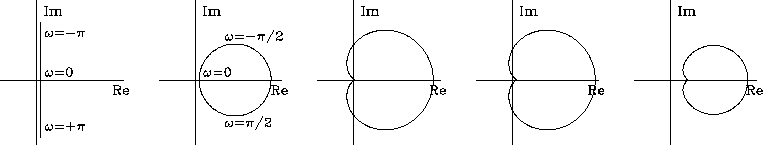 |


The first two panels are explained by the first two functions.
The first two functions and the first two panels look different
but they become the same in the practical limit
of ![]() and
and ![]() .The left panel represents a time derivative in continuous time,
and the second panel likewise
in sampled time is for
a ``causal finite-difference operator''
representing a time derivative.
Notice that the graphs look the same near
.The left panel represents a time derivative in continuous time,
and the second panel likewise
in sampled time is for
a ``causal finite-difference operator''
representing a time derivative.
Notice that the graphs look the same near ![]() .As we sample seismic data with increasing density,
.As we sample seismic data with increasing density,
![]() ,the frequency content shifts further away from the Nyquist frequency.
Measuring
,the frequency content shifts further away from the Nyquist frequency.
Measuring ![]() in radians/sample,
in the limit
in radians/sample,
in the limit
![]() , the physical energy is all near
, the physical energy is all near
![]() .
.
The third panel in Figure 10
shows ![]() which is a cardioid that
wraps itself close up to the negative imaginary axis without touching it.
(To understand the shape near the origin, think about the square
of the leftmost plane. You may have seen examples
of the negative imaginary axis being a branch cut.)
In the fourth panel a small positive quantity kx2 is added which
shifts the cardioid to the right a bit.
Taking the square root gives the last panel
which shows the curve in the right half plane
thus proving
the important result we need,
that
which is a cardioid that
wraps itself close up to the negative imaginary axis without touching it.
(To understand the shape near the origin, think about the square
of the leftmost plane. You may have seen examples
of the negative imaginary axis being a branch cut.)
In the fourth panel a small positive quantity kx2 is added which
shifts the cardioid to the right a bit.
Taking the square root gives the last panel
which shows the curve in the right half plane
thus proving
the important result we need,
that ![]() for all real
for all real ![]() .It is also positive for all real kx because
any kx2>0 shifts the cardioid to the right.
The additional issue of time causality in forward modeling
is covered in IEI.
.It is also positive for all real kx because
any kx2>0 shifts the cardioid to the right.
The additional issue of time causality in forward modeling
is covered in IEI.
Luckily the Fortran csqrt() function assumes the phase of
the argument is between ![]() exactly as we need here.
Thus the square root itself will have a phase between
exactly as we need here.
Thus the square root itself will have a phase between ![]() as we require.
In applications,
as we require.
In applications, ![]() would typically be chosen proportional to the maximum time on the data.
Thus the mathematical expression
would typically be chosen proportional to the maximum time on the data.
Thus the mathematical expression ![]() might be rendered in Fortran as
cmplx(qi,-omega)
where
qi=1./tmax
and the whole concept implemented as in function eiktau()
might be rendered in Fortran as
cmplx(qi,-omega)
where
qi=1./tmax
and the whole concept implemented as in function eiktau() ![[*]](http://sepwww.stanford.edu/latex2html/cross_ref_motif.gif) .
Do not set qi=0 because then the csqrt() function
cannot decipher positive from negative frequencies.
.
Do not set qi=0 because then the csqrt() function
cannot decipher positive from negative frequencies.
complex function eiktau( dt, w, vkx, qi )
real                     dt, w, vkx, qi
eiktau = cexp( - dt * csqrt( cmplx( qi, -w) ** 2   +   vkx * vkx /4. ) )
return; end
Finally, you might ask, why bother with all this careful theory connected with the damped square root. Why not simply abandon the evanescent waves as done by the ``if'' statement in subroutines phasemig() and phasemod()? There are several reasons:
I'm not sure if there is a practical difference between choosing to damp evanescent waves or simply to set them to zero, but there should be a noticable difference on synthetic data: When a Fourier-domain amplitude drops abruptly from unity to zero, we can expect a time-domain signal that spreads widely on the time axis, perhaps dropping off slowly as 1/t. We can expect a more concentrated pulse if we include the evanescent energy, even though it is small. I predict the following behavior: Take an impulse; diffract it and then migrate it. When evanescent waves have been truncated, I predict the impulse is turned into a ``butterfly'' whose wings are at the hyperbola asymptote. Damping the evanescent waves, I predict, gives us more of a ``rounded'' impulse.