Side-boundary analysis

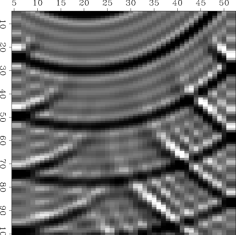
In geophysics, we usually wish the side-boundary question did not arise. The only real reason for side boundaries is that either our survey or our processing activity is necessarily limited in extent. Given that side boundaries are inevitable, we must think about them. The subroutine wavemovie() included zero-slope boundary conditions. This type of boundary treatment resulted from taking

$$\hbox{\tt d(1) = 0. ; d(nx) = 0.}$$

and in the call to ctris taking

$$\hbox{\tt endl = - a ; endr = - c}$$

 

Mexpandsphere90 Figure 5 Given that the domain of computation is $0 \le x \le \$xmax and $0 \le z \le$zmax, how would you modify the initial conditions at z=0 to simulate a point source at (x,z)= (xmax/3, -zmax/2)? (Movie)

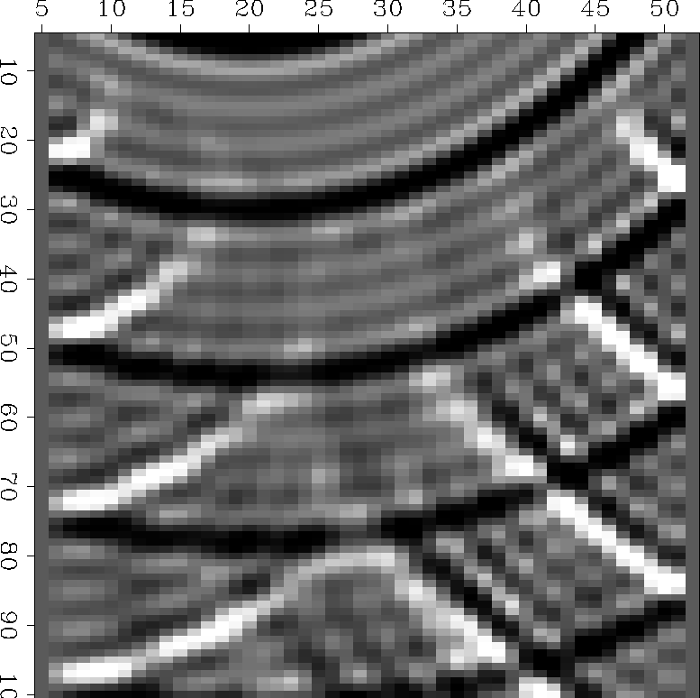
A quick way to get zero-value side-boundary conditions is to take

$$\hbox{\tt endl = endr =}\quad 10^{30} \quad \approx \quad \infty$$

Compare the side-boundary behavior of Figures 5 and 6.

 

Mzeroslope90 Figure 6 Modify the program so that zero-slope side boundaries are replaced by zero-value side boundaries. (Movie)

The zero slope boundary condition is explicitly visible as identical signal on the two end columns. Likewise, the zero-value side boundary condition has a column of zero-valued signal on each side.