Coding a triangle footprint

We should take some care with anti-aliasing in data processing. The anti-aliasing measures we take, however, need not match the field recording. If the field arrays were rectangles, we could use triangles or sincs in the data processing. It happens that triangles are an easy extension of the rectangle work that we have been doing and triangles make a big step in the right direction.

For an input pulse, the output of integration is a step. The output of a second integration is a ramp. For an input triplet (1, 0, 0, -2, 0, 0, 1) the output of two integrations is a short triangle. An easy way to assure time alignment of the triangle center with the triplet center is to integrate once causally and once anticausally as done in subroutine doubint() .  

# Double integration, first causal, then anticausal.
#
subroutine doubint( adj, add, n,             pp   , qq  )
integer             adj, add, n;       real  pp(n), qq(n)
temporary real tt(n)
call adjnull(       adj, add,                pp,n,  qq,n)
if( adj == 0 ) {        call causint( 0,   0, n,pp,  tt  )
                        call causint( 1, add, n,qq,  tt  )
                }
else {                  call causint( 1,   0, n,tt,  qq  )
                        call causint( 0, add, n,tt,  pp  )
                }
return; end

You can imagine placing the ends and apex of each triangle at a nearest neighbor mesh point as we did with the rectangles. Instead I place these ends more precisely on the mesh with linear interpolation. Subroutine lint1() does linear interpolation, but here we need weighted results as provided by spotw() .  

#  Scaled linear interpolation.
#
subroutine spotw( adj, add, scale, nt,t0,dt, t, val,   vec   )
integer it,itc,   adj, add,        nt
real tc, fraction,          scale,    t0,dt, t, val,   vec(nt)
call adjnull(     adj, add,                     val,1, vec,nt)
tc = .5+ (t-t0) / dt;   itc = tc;        it = 1 + itc;  fraction = tc - itc
if( 1 <= it  &&  it < nt) {
        if( adj == 0) {
                vec(it  ) = vec(it  ) + (1.-fraction) * val * scale
                vec(it+1) = vec(it+1) +   fraction    * val * scale
                }
        else
                val = val + ((1.-fraction) * vec(it)  +
                               fraction    * vec(it+1)  ) * scale
        }
else
        call erexit('spotw: at boundary')
return; end

Using these subroutines, I assembled the stacking subroutine tristack() and the NMO routine trimo() with triangle wavelets. The triangle routines are like those for rectangles except for some minor changes. Instead of computing the theoretical locations of impulses on nearer and further traces, I assumed a straight line tangent to the hyperbola $t^2 = \tau^2+x^2/v^2$.Differentiating by x at constant $\tau$ gives the slope dt/dx= x/(v²t). As before, the area of the the wavelets, now triangles must be preserved. The area of a triangle is proportional to the base times the height. Since the triangles are built from double integration ramp functions, the height is proportional to the base length. Thus to preserve areas, each wavelet is scaled by the inverse squared of the triangle's base length. 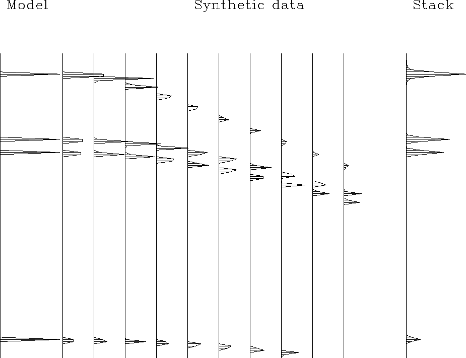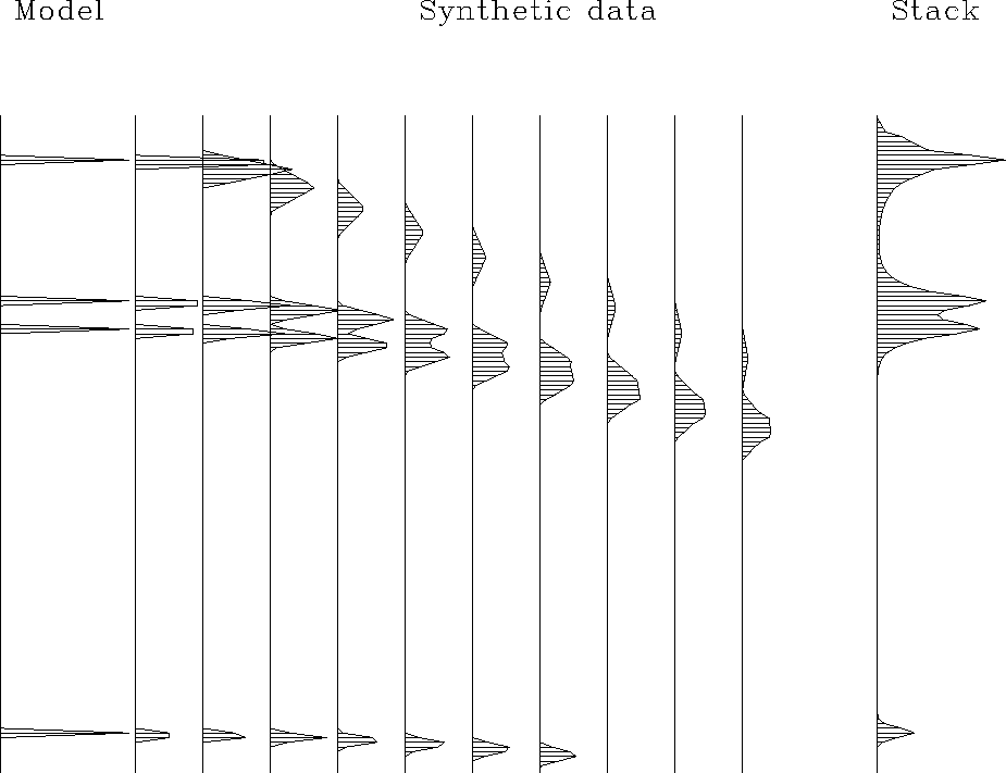Results are shown in Figures 7 and 8.

 

trimo0 Figure 7 Triangle wavelets, accurately positioned, but aliased (antialias=0.)

 

trimo1 Figure 8 Antialiased triangle wavelets. (antialias=1.) Where ever triangle duration is more than about three points, the end of one triangle marks the apex of the next.

 

# Modeling and stacking using triangle weighted moveout.
#
subroutine tristack( adj,add, slow,anti,t0,dt,x0,dx, nt,nx, stack, gather   )
integer ix,          adj,add,                        nt,nx
real x,                    slow(nt),anti,t0,dt,x0,dx, stack(nt), gather(nt,nx)
call adjnull(        adj, add,                        stack,nt,  gather,nt*nx)
do ix= 1, nx {  x =  x0 + dx * (ix-1)
        call trimo( adj,1,t0,dt,dx, x, nt,slow,0.,1.,anti,stack, gather(1,ix))
        }
return; end

 

# moveout with triangle shaped smoothing window.
#
subroutine trimo(  adj, add, t0,dt, dx,x, nt, slow, s02, wt, anti, zz,    tt )
integer iz,itp,itm,adj, add,              nt
real                         t0,dt, dx,x, slow(nt), s02, wt, anti, zz(nt),tt(nt)
real z, t,tm,tp, amp, slope
temporary real ss(nt)
call null(     ss,nt);  call adjnull( adj, add,                    zz,nt, tt,nt)
if( adj != 0 )          call doubint( 1, 0, nt, ss, tt)
do iz= 2, nt {  z = t0 + dt * (iz-1)
        t = sqrt( z**2 + (slow(iz) * x)**2 )
        slope = anti * ( slow(iz)**2 - s02 ) * x / t
        tp = t + abs(slope * dx) + dt;   itp = 1.5 + (tp-t0) / dt
        tm = t - abs(slope * dx) - dt;   itm = 1.5 + (tm-t0) / dt
        if( itm <= 1  )  next
        if( itp >= nt )  break
        amp = wt * sqrt( nt*dt/t) * z/t * (dt/(dt+tp-tm)) ** 2
        call spotw( adj, 1,  -amp, nt,t0,dt,tm, zz(iz), ss)
        call spotw( adj, 1, 2*amp, nt,t0,dt,t , zz(iz), ss)
        call spotw( adj, 1,  -amp, nt,t0,dt,tp, zz(iz), ss)
        }
if( adj == 0)           call doubint( 0, add, nt, ss, tt)
return; end

From the stack reconstruction of the model in Figure 8 we see the reconstruction is more blured with antialiasing than it was without in Figure 7. The benefit of antialiasing will become clear next in more complicated examples where events cross.