![[*]](http://sepwww.stanford.edu/latex2html/cross_ref_motif.gif) equation (
equation (![[*]](http://sepwww.stanford.edu/latex2html/cross_ref_motif.gif) )
)
With velocity analysis, we estimate the RMS velocity.
Later we will need both the RMS velocity and the interval velocity.
(The word ``interval'' designates an interval between two reflectors.)
Recall from chapter ![[*]](http://sepwww.stanford.edu/latex2html/cross_ref_motif.gif) equation (
equation (![[*]](http://sepwww.stanford.edu/latex2html/cross_ref_motif.gif) )
)
![]()
Routine vint2rms() ![[*]](http://sepwww.stanford.edu/latex2html/cross_ref_motif.gif) converts from interval velocity to RMS velocity
and vice versa.
converts from interval velocity to RMS velocity
and vice versa.
# Invertible transform from interval velocity to RMS.
#
subroutine vint2rms(  inverse, vminallow, dt, vint, nt,  vrms )
integer it, wide,     inverse,                      nt
real    vmin,                  vminallow, dt, vint( nt), vrms( nt)
temporary real                                 vis( nt),  sum( nt)
if( inverse == 0) {             do it= 1, nt
                                        vis(it) = vint(it) ** 2
        sum(1) = 0.;            do it= 2, nt
                                        sum(it) = sum(it-1) + vis(it) * dt
        vrms(1) = vint(1);      do it= 2, nt
                                        vrms(it) = sqrt( sum(it) / ((it-1)*dt) )
        }
else {  do it= 1, nt
                sum(it)= ((it-1)*dt) * amax1( vrms(it)**2, vminallow**2 )
        vis(1) = vrms(1) ** 2
        do it= 2, nt
                vis(it) = ( sum(it) - sum(it-1) )/ dt
        wide= 2;  repeat {
                vmin = vis(1);  do it=1,nt { if( vis(it)<vmin)  vmin = vis(it) }
                if( vmin > vminallow**2 )   break
                call triangle( wide, 1, nt, vis, vis)           # smooth vis()
                wide = wide + 1
                if( wide >= nt/3) call erexit('Velocity less than allowable.')
                }
        do it= 1, nt
                vint(it) = sqrt( vis(it))
        }
return; end
The forward conversion follows
in straightforward steps: square, integrate, square root.
The inverse conversion, like an adjoint,
retraces the steps of the forward transform
but it does the inverse at every stage.
There is however,
a messy problem with nearly all field data
that must be handled along the inverse route.
The problem is that the observed RMS velocity function
is generally a rough function,
and it is generally unreliable over a significant portion of its range.
To make matters worse,
deriving an interval velocity begins as does a derivative,
roughening the function further.
We soon find ourselves taking square roots of negative numbers,
which requires judgement to proceed.
The technique used in vint2rms() ![[*]](http://sepwww.stanford.edu/latex2html/cross_ref_motif.gif) is to average the squared interval velocity
in ever expanding neighborhoods until there are no longer
any negative squared interval velocities.
As long as we are restricting v2 from being negative,
it is easy to restrict it to be above some allowable velocity,
say vminallow.
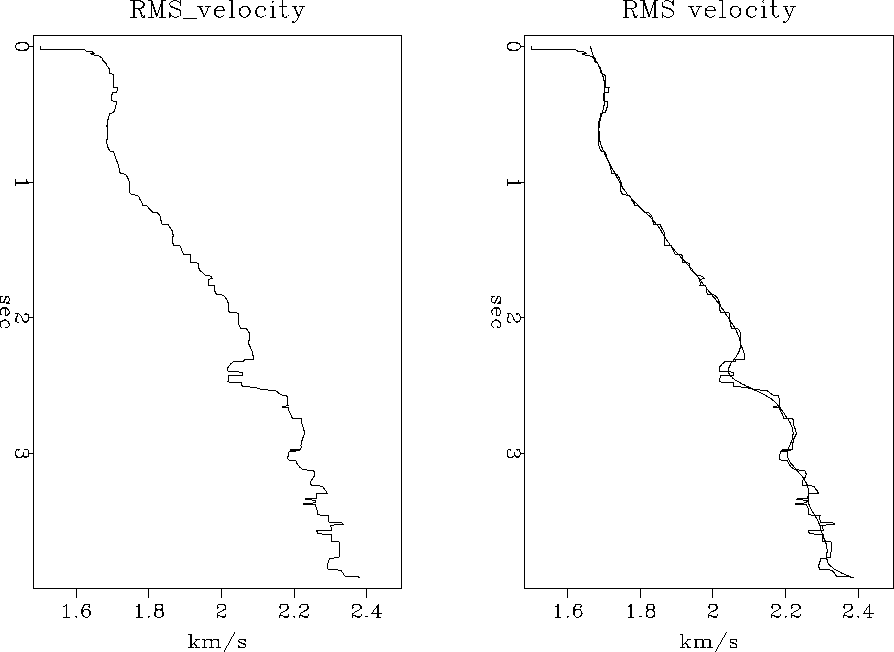
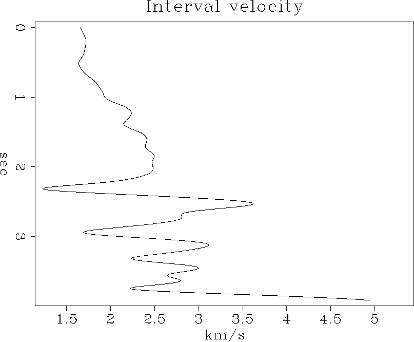
Figures 11 and 12
were derived from the velocity scans in Figure 10.
is to average the squared interval velocity
in ever expanding neighborhoods until there are no longer
any negative squared interval velocities.
As long as we are restricting v2 from being negative,
it is easy to restrict it to be above some allowable velocity,
say vminallow.
Figures 11 and 12
were derived from the velocity scans in Figure 10.
 |
![[*]](http://sepwww.stanford.edu/latex2html/cross_ref_motif.gif) .
The interval velocity associated with the smoothed velocity
is in figure 12.
.
The interval velocity associated with the smoothed velocity
is in figure 12.
|
vrmsint
Figure 12 Interval velocity associated with the smoothed RMS velocity of Figure 11. Pushbutton allows experimentation with vminallow. |  |