


Z transforms and Fourier transforms are related
by the relations ![]() and
and
![]() .A problem with these relations is that
simple ratios of polynomials in Z do not translate to
ratios of polynomials in
.A problem with these relations is that
simple ratios of polynomials in Z do not translate to
ratios of polynomials in ![]() and vice versa. The
approximation
and vice versa. The
approximation
| |
(42) |
| |
(43) |
| |
(44) |
| |
(45) |
For a Z transform B(Z) to be minimum phase,
any root Z0 of 0 = B(Z0) should be outside the
unit circle. Since
![]() and
and ![]() , it means
that for a minimum phase
, it means
that for a minimum phase ![]() should be
negative. (In other words,
should be
negative. (In other words, ![]() is in the lower
half-plane.) Thus it may be said that
is in the lower
half-plane.) Thus it may be said that
![]() maps the exterior of the unit circle
to the lower half-plane. By inspection of
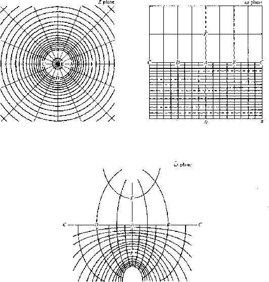
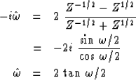
Figures 20 and 21, it is found
that the bilinear approximation (42) or
(43) also maps the exterior of the unit
circle into the lower half-plane.
maps the exterior of the unit circle
to the lower half-plane. By inspection of
Figures 20 and 21, it is found
that the bilinear approximation (42) or
(43) also maps the exterior of the unit
circle into the lower half-plane.
|
2-20
Figure 20 Some typical points in the Z-plane, the | 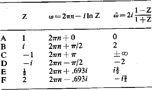 |

 |
Thus, although the bilinear approximation is an approximation, it turns out to exactly preserve the minimum-phase property. This is very fortunate because if a stable differential equation is converted to a difference equation via (42), the resulting difference equation will be stable. (Many cases may be found where the approximation of a time derivative by multiplication with 1 - Z would convert a stable differential equation into an unstable difference equation.)
A handy way to remember (42) is that
![]() corresponds to time differentiation
of a Fourier transform and (1 - Z) is the
first differencing operator. The (1 + Z) in
the denominator gets things ``centered" at
Z1/2
corresponds to time differentiation
of a Fourier transform and (1 - Z) is the
first differencing operator. The (1 + Z) in
the denominator gets things ``centered" at
Z1/2
To see that the bilinear approximation is a low-frequency approximation, multiply top and bottom of (42) by Z-1/2
 |
||
| (46) |
| |
(47) |
|
2-22
Figure 22 The accuracy of the bilinear transformation approximation. | 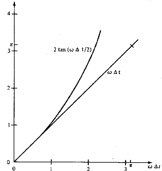 |
From Figure 22 we see that the
error will be only a few percent if we choose
![]() small enough so that
small enough so that
![]() . Readers
familiar with the folding theorem will recall
that it gives the less severe restraint
. Readers
familiar with the folding theorem will recall
that it gives the less severe restraint
![]() . Clearly,
the folding theorem is too generous for
applications involving the bilinear transform.
. Clearly,
the folding theorem is too generous for
applications involving the bilinear transform.
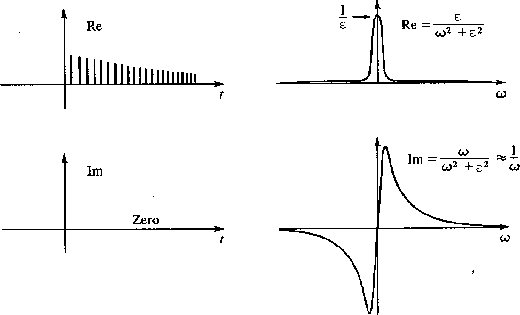
Now, by way of example, let us take up the case
of a pole ![]() at zero frequency.
This is integration. For reasons which will presently
be clear, we will consider the slightly different pole
at zero frequency.
This is integration. For reasons which will presently
be clear, we will consider the slightly different pole
| |
(48) |
![\begin{eqnarray}
P
&= & {1 \over 2 [(1 - Z)/(1 + Z)] + \varepsilon}
\eq {0.5(1...
...& {0.5(1 + Z) \over (1 + \varepsilon /2)
- Z(1 - \varepsilon /2)}\end{eqnarray}](img136.gif) |
||
| (49) |
 |