


Next: UP- AND DOWNGOING WAVES
Up: Mathematical physics in stratified
Previous: FROM PHYSICS TO MATHEMATICS
A differential equation relates field variables at a point to field variables at neighboring points.
A matrizant relates field variables at one depth in a stratified material to variables at some other depth.
A matrizant may also be regarded as the integral of the matrix differential equation (9-1-7).
First we will show how to get the matrizant of (9-1-7) by numerical means.
That is, we will solve the problem for arbitrary depth variations
in density and in compressibility.
Then we will come back and develop analytical solutions
for the special case of constant material properties.
We have

or
|  |
(1) |
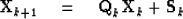
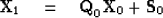
Given  for some particular z it is clear that (9-2-1) may be used recursively to get for any z.
For simplicity we may take
for some particular z it is clear that (9-2-1) may be used recursively to get for any z.
For simplicity we may take  and use subscripts to indicate the z coordinate.
Let
and use subscripts to indicate the z coordinate.
Let ![$[\mbox{\bf I} + \mbox{\bf A}(z)\triangle z]$](img51.gif) be denoted by
be denoted by  ,then (9-2-1) becomes
or
hence
hence
likewise
|  |
(2) |
So we have in general a numerically determinable matrix  (called the matrizant)
and a vector
(called the matrizant)
and a vector  which relates the field variables
at the top of the strata to those on the bottom by
which relates the field variables
at the top of the strata to those on the bottom by
|  |
(3) |
The matrix is also called an integral matrix.
Physical problems present themselves in different ways with different boundary conditions.
For the acoustic problem discussed earlier is a two-component vector involving pressure and of the stratified medium.
Thus (9-2-3) represents two equations for four unknowns.
The solution to the problem comes only when two boundary conditions are introduced.
If we are talking about sound waves in the ocean,
(simplified) boundary conditions would be to prescribe zero pressure at the surface and zero vertical displacement at the sea floor.
Then these boundary conditions with (9-2-3)
would be two equations and two unknowns
and consequently could be solved for surface displacement and bottom pressure.
From these,
pressure and displacement could be determined everywhere.
Proper determination of boundary conditions
is often the trickiest part of a problem;
we will return to it for some other problems in a later section.
If portions of the material have constant material properties
and contain no sources,
then it is possible to find an analytical expression for the matrizant.
A matrizant which takes one across such a layer of constant properties
is called, appropriately enough, a layer matrix.
It may be verified by substitution that
| ![\begin{displaymath}
\mbox{\bf X}_{z} \eq e^{[\mbox{\bf A}(z-z_{0})]}\mbox{\bf X}_{z_{0}}\end{displaymath}](img61.gif) |
(4) |
is the solution to 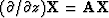 where
where
| 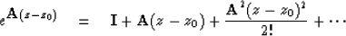 |
(5) |
in a region of space where  is constant with z.
Thus
is constant with z.
Thus  is the required matrizant.
The matrix exponential could be computed
numerically either by the method of (9-2-2) or the method of (9-2-5)
or the method of Sylvester's theorem described in Chap. 5.
In the next section we will see how Sylvester's theorem
leads directly to the ideas of up- and downgoing waves.
is the required matrizant.
The matrix exponential could be computed
numerically either by the method of (9-2-2) or the method of (9-2-5)
or the method of Sylvester's theorem described in Chap. 5.
In the next section we will see how Sylvester's theorem
leads directly to the ideas of up- and downgoing waves.
EXERCISES:
-
What is
 for the improved central difference approximation?
![\begin{displaymath}
\mbox{\bf X}(z + \triangle z) - \mbox{\bf X}(z) \eq \frac{\t...
...ox{\bf A}[\mbox{\bf X}(z + \triangle z) + \mbox{\bf X}(z)]}{2} \end{displaymath}](img66.gif)
Next: UP- AND DOWNGOING WAVES
Up: Mathematical physics in stratified
Previous: FROM PHYSICS TO MATHEMATICS
Stanford Exploration Project
10/30/1997