FINITE DIFFERENCES ON A HELIX

The function  

$$\mathcal r \eq \begin{array} {\vert r\vert r\vert r\vert r\v... ...line -1&0&\cdots&0&-1&4&-1&0& \cdots&0&-1 \\ \hline\end{array}$$ (8)

is an autocorrelation function. It is symmetrical about the ``4'' and its Fourier transform is positive for all frequencies. Digging out our old textbooks we discover how to compute a causal wavelet with this autocorrelation. I used the ``Kolmogoroff spectral-factorization method'' to find this wavelet $\mathcal h$: 

$${\mathcal h} \eq \begin{array} {\vert r\vert r\vert r\vert r... ....024&\cdots&\cdots&-.044&-.087&-.200&-.558 \\ \hline\end{array}$$ (9)

According to the Kolmogoroff theory, if we form the autocorrelation of $\mathcal h$,we will get $\mathcal r$.This is not obvious from the numbers themselves because the computation requires a little work.

Let the time reversed version of $\mathcal h$be denoted $\mathcal h'$.This notation is consistant with an idea from Chapter that the adjoint of a filter matrix is another filter matrix with a reversed filter. In engineering it is conventional to use the asterisk symbol ``$\ast$'' to denote convolution. Thus, the idea that the autocorrelation of a signal $\mathcal h$is a convolution of the signal $\mathcal h$with its time reverse (adjoint) can be written as $\mathcal h' \ast \mathcal h = \mathcal h \ast \mathcal h' = \mathcal r$.

Wind the signal $\mathcal r$ around a vertical-axis helix to see its two-dimensional shape $\mathcal R$: 

$$\mathcal r \quad \xrightarrow{\rm helical \; boundaries} \qu... ... -1 & 4 & -1\\ \hline & -1 & \\ \hline\end{array}\eq \mathcal R$$ (10)

This 2-D filter is the negative of the finite-difference representation of the Laplacian operator, generally denoted $\nabla^2= {\partial^2\over \partial x^2} + {\partial^2\over \partial y^2}$.Now for the magic: Wind the signal $\mathcal h$ around the same helix to see its two-dimensional shape $\mathcal H$ 

$${\mathcal H} \eq \begin{array} {\vert r\vert r\vert r\vert ... ...&-.044 & -.087 & -.200 & -.558 & & & & \\ \hline \end{array}$$ (11)

In the representation (11) we see the coefficients diminishing rapidly away from maximum value 1.791. My claim is that the two-dimensional autocorrelation of (11) is (10). You verified this idea earlier when the numbers were all ones. You can check it again in a few moments if you drop the small values, say 0.2 and smaller.

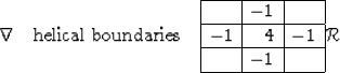
Since the autocorrelation of $\mathcal H$ is $\mathcal H' \ast \mathcal H = \mathcal R =-\nabla^2$is a second derivative, the operator $\mathcal H$ must be something like a first derivative. As a geophysicist, I found it natural to compare the operator ${\partial\over\partial y}$with $\mathcal H$ by applying them to a local topographic map. The result shown in Figure is that $\mathcal H$ enhances drainage patterns whereas ${\partial\over\partial y}$ enhances mountain ridges.

 

helocut90
Figure 7 Topography, helical derivative, slope south.

The operator $\mathcal H$ has curious similarities and differences with the familiar gradient and divergence operators. In two-dimensional physical space, the gradient maps one field to two fields (north slope and east slope). The factorization of $-\nabla^2$ with the helix gives us the operator $\mathcal H$that maps one field to one field. Being a one-to-one transformation (unlike gradient and divergence) the operator $\mathcal H$ is potentially invertible by deconvolution (recursive filtering).

I have chosen the name ``helix derivative'' or ``helical derivative'' for the operator $\mathcal H$.A telephone pole has a narrow shadow behind it. The helix integral (middle frame of Figure ) and the helix derivative (left frame) show shadows with an angular bandwidth approaching $180^\circ$.

Our construction makes $\mathcal H$ have the energy spectrum k_x²+k_y², so the magnitude of the Fourier transform is $\sqrt{k_x^2+k_y^2}$.It is a cone centered and with value zero at the origin. By contrast, the components of the ordinary gradient have amplitude responses |k_x| and |k_y| that are lines of zero across the (k_x,k_y)-plane.

The rotationally invariant cone in the Fourier domain contrasts sharply with the nonrotationally invariant function shape in (x,y)-space. The difference must arise from the phase spectrum. The factorization (11) is nonunique in that causality associated with the helix mapping can be defined along either x- or y-axes; thus the operator (11) can be rotated or reflected.

This is where the story all comes together. One-dimensional theory, either the old Kolmogoroff spectral factorization, or the new Wilson-Burg spectral-factorization method produces not merely a causal wavelet with the required autocorrelation. It produces one that is stable in deconvolution. Using $\mathcal H$ in one-dimensional polynomial division, we can solve many formerly difficult problems very rapidly. Consider the Laplace equation with sources (Poisson's equation). Polynomial division and its reverse (adjoint) gives us $\mathcal p =(\mathcal q/\mathcal H)/\mathcal H'$which means that we have solved $\nabla^2 \mathcal p = -\mathcal q$by using polynomial division on a helix. Using the seven coefficients shown, the cost is fourteen multiplications (because we need to run both ways) per mesh point. An example is shown in Figure .

 

lapfac90
Figure 8 Deconvolution by a filter whose autocorrelation is the two-dimensional Laplacian operator. Amounts to solving the Poisson equation. Left is $\mathcal q$; Middle is $\mathcal q/\mathcal H$; Right is $(\mathcal q/\mathcal H)/\mathcal H'$.

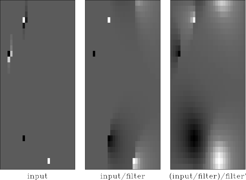Figure contains both the helix derivative and its inverse. Contrast them to the x- or y-derivatives (doublets) and their inverses (axis-parallel lines in the (x,y)-plane). Simple derivatives are highly directional whereas the helix derivative is only slightly directional achieving its meagre directionality entirely from its phase spectrum.

In practice we often require an isotropic filter. Such a filter is a function of $k_r=\sqrt{k_x^2 + k_y^2}$.It could be represented as a sum of helix derivatives to integer powers.

 

• Matrix view of the helix