

Next: Variance of the sample
Up: TIME-STATISTICAL RESOLUTION
Previous: Probability and independence
Now let xt be a time series made up of identically distributed
random numbers: mx and  do not depend on time.
Let us also suppose that they are independently chosen; this
means in particular that for any different times t and s (
 ):
):
|  |
(13) |
Suppose we have a sample of n points of xt and are
trying to determine the value of mx.
We could make an estimate  of the mean mx with the formula
|  |
(14) |
A somewhat more elaborate method of estimating the mean
would be to take a weighted average.
Let wt define a set of weights normalized so that
|  |
(15) |
With these weights, the more elaborate estimate  of the mean is
|  |
(16) |
Actually (14) is just a special case of (16);
in (14) the
weights are wt = 1/n.
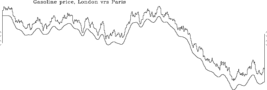
Further, the weights could be convolved on the random time series,
to compute local averages of this time series, thus smoothing it.
The weights are simply a filter response where the filter coefficients happen
to be positive and cluster together.
Figure 6 shows an example: a random walk function
with itself smoothed locally.
walk
Figure 6
Random walk and itself smoothed (and shifted downward).


Next: Variance of the sample
Up: TIME-STATISTICAL RESOLUTION
Previous: Probability and independence
Stanford Exploration Project
3/1/2001
