BOTH MISSING DATA AND UNKNOWN FILTER

Recall the missing-data figures beginning with Figure . There the filters were taken as known, and the only unknowns were the missing data. Now, instead of having a predetermined filter, we will solve for the filter along with the missing data. The principle we will use is that the output power is minimized while the filter is constrained to have one nonzero coefficient (else all the coefficients would go to zero). We will look first at some results and then see how they were found.

 

misif90 Figure 10 Top is known data. Middle includes the interpolated values. Bottom is the filter with the leftmost point constrained to be unity and other points chosen to minimize output power.

In Figure 10 the filter is constrained to be of the form (1,a₁,a₂). The result is pleasing in that the interpolated traces have the same general character as the given values. The filter came out slightly different from the (1,0,-1) that I guessed and tried in Figure . Curiously, constraining the filter to be of the form (a_-2,a_-1,1) in Figure 11 yields the same interpolated missing data as in Figure 10. I understand that the sum squared of the coefficients of A(Z)P(Z) is the same as that of A(1/Z)P(Z), but I do not see why that would imply the same interpolated data; never the less, it seems to.

 

backwards90 Figure 11 The filter here had its rightmost point constrained to be unity--i.e., this filtering amounts to backward prediction. The interpolated data seems to be identical to that of forward prediction.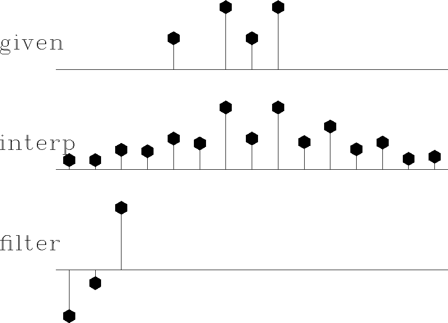