 |
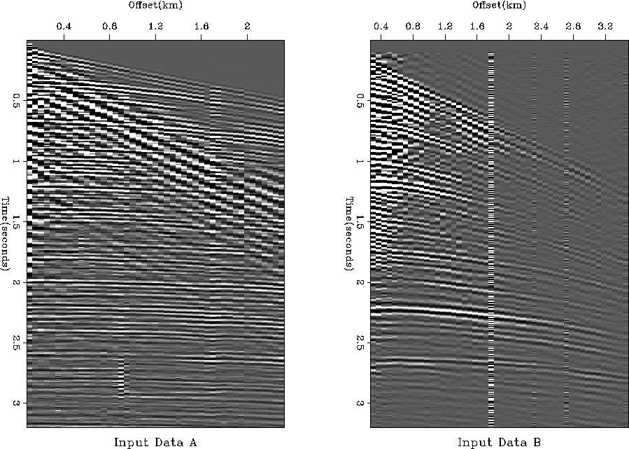
Figure 9 Input data- 2 CMP gathers.
 |
Figure 9 displays different interesting features: the first
CMP (![]() ) shows low velocity events (ground roll or guided waves) and time
shifts near offset 2km while the second example (B) shows bad traces with high amplitudes.
The same clip has been applied to each figure.
Note that the offsets are probably wrong since we have reflected waves traveling at about 10 km/s for
Input A!
) shows low velocity events (ground roll or guided waves) and time
shifts near offset 2km while the second example (B) shows bad traces with high amplitudes.
The same clip has been applied to each figure.
Note that the offsets are probably wrong since we have reflected waves traveling at about 10 km/s for
Input A!
 |
 |
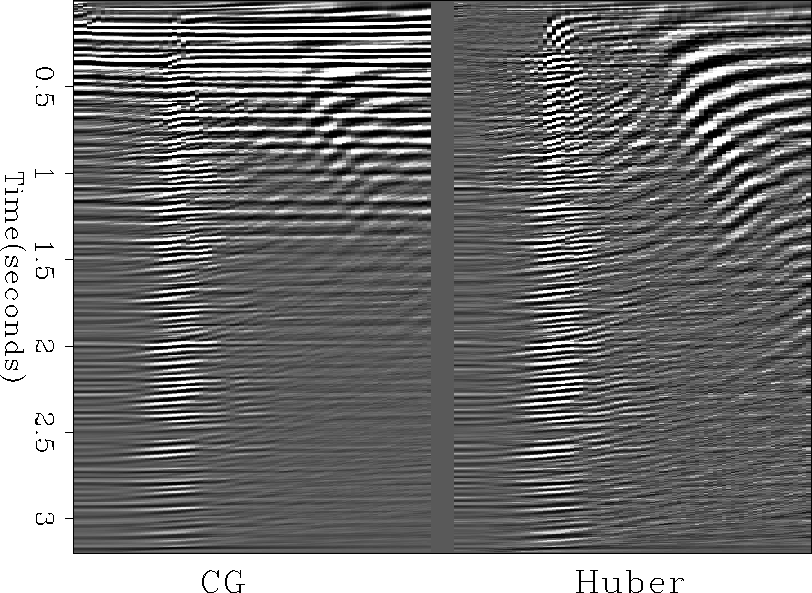
The velocities are computed after 5 iterations only, and ![]() for both
gathers. Figure10 shows the velocity analysis using Huber and CG on a first data set.
It appears that the CG result has artifacts at times above 1.5 sec. We see some horizontal stripes
that make reliable interpretation difficult. In contrast, the Huber result displays a
focused velocity corridor. Some low frequency events do appear in the upper right part of the panel
but they do not interfere with the main fairway. It is interesting to notice
that Huber separates the low-frequency low-velocity
noise from the signal whereas the l2 measure spreads it along the velocity axis.
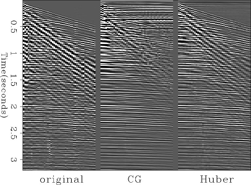
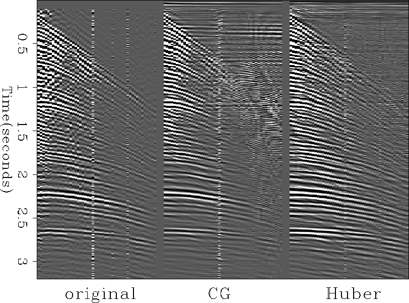
If we now model those results back into the data-space, we obtain Figure11.
We notice that CG does not do a good job in estimating the upper part. Furthermore, some high frequency
noise appears. The Huber result however looks close to the original data. In particular, the upper part
is well estimated and no harmful artifacts are visible.
The anomalous high amplitude first trace does not affect the final results either.
for both
gathers. Figure10 shows the velocity analysis using Huber and CG on a first data set.
It appears that the CG result has artifacts at times above 1.5 sec. We see some horizontal stripes
that make reliable interpretation difficult. In contrast, the Huber result displays a
focused velocity corridor. Some low frequency events do appear in the upper right part of the panel
but they do not interfere with the main fairway. It is interesting to notice
that Huber separates the low-frequency low-velocity
noise from the signal whereas the l2 measure spreads it along the velocity axis.
If we now model those results back into the data-space, we obtain Figure11.
We notice that CG does not do a good job in estimating the upper part. Furthermore, some high frequency
noise appears. The Huber result however looks close to the original data. In particular, the upper part
is well estimated and no harmful artifacts are visible.
The anomalous high amplitude first trace does not affect the final results either.
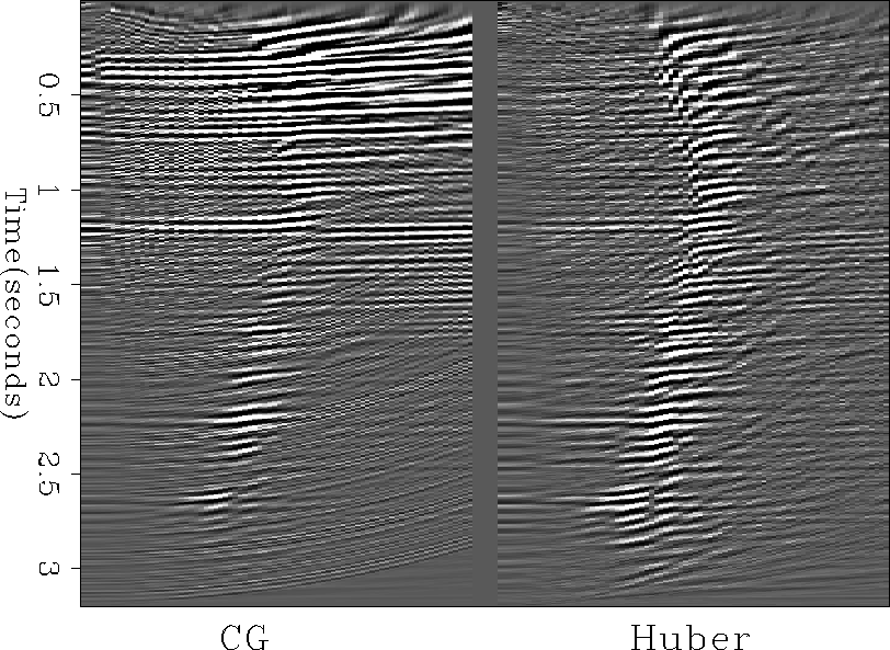
Let's now look at the results for Input B. Figure12 show the strength of the Huber solver compared to CG. The CG velocity panel shows horizontal stripes in the velocity scan making any reliable picking quite impossible. The Huber velocity panel displays a focused bended corridor with low noise amplitude. If we now model those results back into the data-space, we get Figure13. Those sections support the same observations as previous, and as expected, Huber allows to recover more accurately the original data. These results are quite encouraging and give us a flavor of what could be accomplished with the Huber norm. The same conclusion applies on the field data as on the synthetics: the Huber function is robust.
 |
 |