

Next: Conclusions
Up: Fomel: Velocity continuation
Previous: Putting together prestack velocity
After the velocity continuation process has created a velocity cube in
the prestack common-offset migration domain, we can pick the best
focusing velocity from that cube. To automatize the velocity picking
procedure, I have designed a simple algorithm. The algorithm based on
solving the following regularized least-square system:
|  |
(7) |
Here  are blind maximum-semblance picks (possibly in a
predefined fairway),
  is the estimated velocity picks,
 is the weighting operator with the weight corresponding to
the semblance values at
  ,
,  is a roughening
operator, and
  is the scalar regularization parameter. The
first least-square fitting goal in (7) states that the
estimated velocity picks should match the measured picks where the
semblance is high enough
is the scalar regularization parameter. The
first least-square fitting goal in (7) states that the
estimated velocity picks should match the measured picks where the
semblance is high enough![[*]](http://sepwww.stanford.edu/latex2html/foot_motif.gif) .
The second fitting goal tries to find the smoothest velocity function
possible. The least-square solution of problem (7) takes
the form
.
The second fitting goal tries to find the smoothest velocity function
possible. The least-square solution of problem (7) takes
the form
|  |
(8) |
where  denotes the adjoint operator. In the case of
picking a one-dimensional velocity function from a single semblance
panel, we can simplify the algorithm by choosing
  to be the
a convolution with the derivative filter (1,-1). It is easy to
notice that in this case the inverted matrix in formula (8)
has a tridiagonal structure and therefore can be easily inverted with
a linear-time algorithm. The regularization parameter
  controls the amount of smoothing of the estimated velocity function.
Figure
 ![[*]](http://sepwww.stanford.edu/latex2html/cross_ref_motif.gif) shows a velocity spectrum and two automatic
picks for different values of
shows a velocity spectrum and two automatic
picks for different values of  .
velpick
Figure 4 Semblance panel (left) and automatic
velocity picks for different values of the regularization parameter.
Center:  , right:
  . Higher values of
 lead to smoother velocities.


In the case of picking two- or three-dimensional velocity functions,
one could generalize problem (7) by defining  as a 2-D or 3-D roughening operator. I chose to use a more simplistic
approach. I transform system (7) to the form
|  |
(9) |
where  is still one-dimensional, and
  is the
estimate from the previous midpoint location. The scalar parameter
 controls the amount of lateral continuity in the estimated
velocity function. The least-square solution to system
(9) takes the form:
|  |
(10) |
where  denotes the identity matrix. Formula (10)
also reduces to an efficient tridiagonal matrix inversion.
Figure
 ![[*]](http://sepwww.stanford.edu/latex2html/cross_ref_motif.gif) shows a result of two-dimensional velocity
picking after velocity continuation. I used values of
shows a result of two-dimensional velocity
picking after velocity continuation. I used values of  and
and  . The first parameter controls the vertical smoothing
of velocities, while the second parameter controls the amount of
lateral continuity.
beifpk
Figure 5 Automatic picks of 2-D RMS velocity
after velocity continuation. The contour spacing is 0.1 km/s, starting
from 1.5 km/s.


Figure ![[*]](http://sepwww.stanford.edu/latex2html/cross_ref_motif.gif) shows the final result of velocity
continuation: an image, obtained by slicing through the velocity cube
with the picked RMS velocity. Different parts of the image have been
properly positioned and focused by the velocity continuation process.
One way to further improve the image quality is hybrid
migration : demigration to zero-offset, followed by post-stack depth
migration Kim et al. (1997). This step requires constructing
an interval velocity model from the picked RMS velocities.
shows the final result of velocity
continuation: an image, obtained by slicing through the velocity cube
with the picked RMS velocity. Different parts of the image have been
properly positioned and focused by the velocity continuation process.
One way to further improve the image quality is hybrid
migration : demigration to zero-offset, followed by post-stack depth
migration Kim et al. (1997). This step requires constructing
an interval velocity model from the picked RMS velocities.
beifmg
Figure 6 Final result of
velocity continuation: seismic image, obtained by slicing through
the velocity cube.


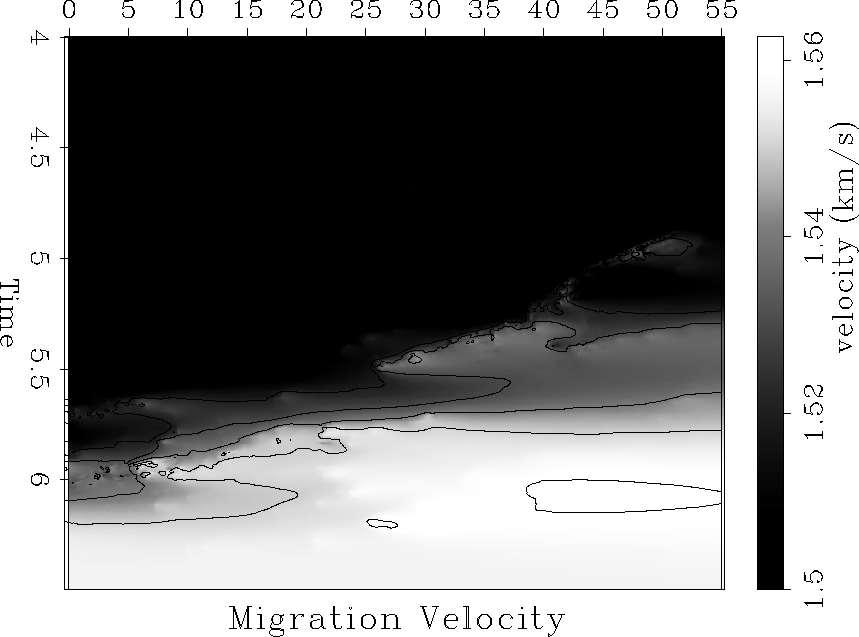
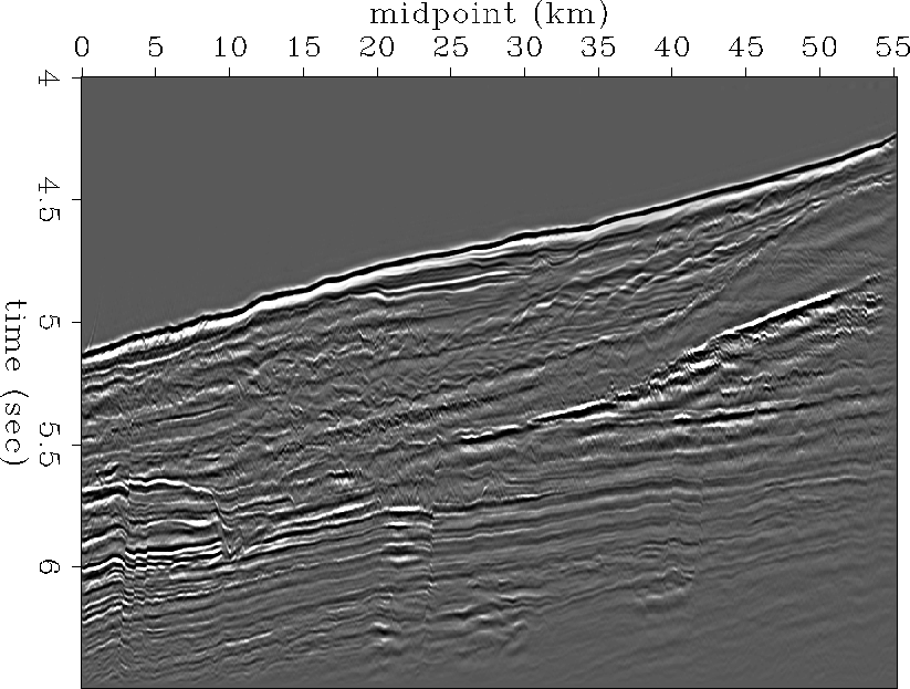
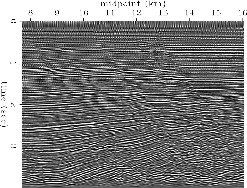
Without repeating the details of the procedure, Figures ![[*]](http://sepwww.stanford.edu/latex2html/cross_ref_motif.gif) and
and ![[*]](http://sepwww.stanford.edu/latex2html/cross_ref_motif.gif) show picked RMS velocities and the velocity
continuation image for the Blake Outer Ridge data, shown in many other
papers in this report.
show picked RMS velocities and the velocity
continuation image for the Blake Outer Ridge data, shown in many other
papers in this report.
pck
Figure 7 Blake Outer Ridge data. Automatic
picks of 2-D RMS velocity after velocity continuation. The contour
spacing is 0.01 km/s, starting from 1.5 km/s.


 img
img
Figure 8 Blake Outer Ridge
data. Final result of velocity continuation: seismic image, obtained
by slicing through the velocity cube.


Next: Conclusions
Up: Fomel: Velocity continuation
Previous: Putting together prestack velocity
Stanford Exploration Project
4/20/1999
![[*]](http://sepwww.stanford.edu/latex2html/foot_motif.gif) .
The second fitting goal tries to find the smoothest velocity function
possible. The least-square solution of problem (7) takes
the form
.
The second fitting goal tries to find the smoothest velocity function
possible. The least-square solution of problem (7) takes
the form
![[*]](http://sepwww.stanford.edu/latex2html/cross_ref_motif.gif) shows a velocity spectrum and two automatic
picks for different values of
shows a velocity spectrum and two automatic
picks for different values of 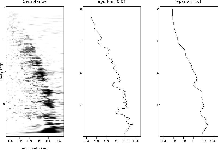
![]() as a 2-D or 3-D roughening operator. I chose to use a more simplistic
approach. I transform system (7) to the form
as a 2-D or 3-D roughening operator. I chose to use a more simplistic
approach. I transform system (7) to the form

![[*]](http://sepwww.stanford.edu/latex2html/cross_ref_motif.gif) shows a result of two-dimensional velocity
picking after velocity continuation. I used values of
shows a result of two-dimensional velocity
picking after velocity continuation. I used values of 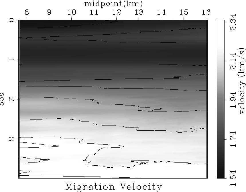
![[*]](http://sepwww.stanford.edu/latex2html/cross_ref_motif.gif) shows the final result of velocity
continuation: an image, obtained by slicing through the velocity cube
with the picked RMS velocity. Different parts of the image have been
properly positioned and focused by the velocity continuation process.
One way to further improve the image quality is hybrid
migration : demigration to zero-offset, followed by post-stack depth
migration Kim et al. (1997). This step requires constructing
an interval velocity model from the picked RMS velocities.
shows the final result of velocity
continuation: an image, obtained by slicing through the velocity cube
with the picked RMS velocity. Different parts of the image have been
properly positioned and focused by the velocity continuation process.
One way to further improve the image quality is hybrid
migration : demigration to zero-offset, followed by post-stack depth
migration Kim et al. (1997). This step requires constructing
an interval velocity model from the picked RMS velocities.
![[*]](http://sepwww.stanford.edu/latex2html/cross_ref_motif.gif) and
and ![[*]](http://sepwww.stanford.edu/latex2html/cross_ref_motif.gif) show picked RMS velocities and the velocity
continuation image for the Blake Outer Ridge data, shown in many other
papers in this report.
show picked RMS velocities and the velocity
continuation image for the Blake Outer Ridge data, shown in many other
papers in this report.
