|
noah2d
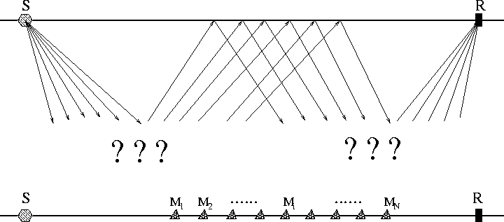
Figure 4 2-D multiple prediction. All the contributing traces form a 2-D MCG prior to summation. The question marks in the plot indicate that the underground structures are unknown. |  |
Figure 4 schematically demonstrates 2-D multiple prediction. In order to predict the multiple from source S to receiver R, we need to cross-convolute all the possible contributing traces marked by Mi in the middle, since we do not know where exactly the multiple reflection occurs on the surface. Then the summation step locates the exact multiple reflection position as long as the contributing traces are densely sampled on the surface.
|
noah2d
Figure 4 2-D multiple prediction. All the contributing traces form a 2-D MCG prior to summation. The question marks in the plot indicate that the underground structures are unknown. |  |
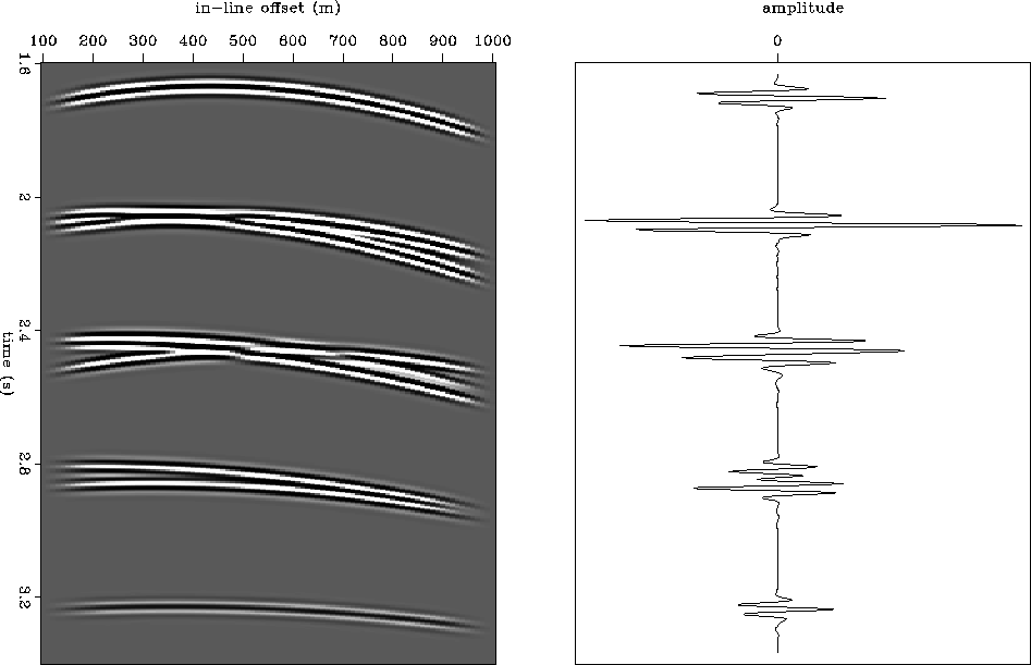
Prior to summation, if we lay out the cross-convoluted traces from left to right, we get an intermediate result, a multiple contribution gather (MCG). Figure 5 shows a 2-D multiple contribution gather and the corresponding summation result. The MCG is a section in 2-D and a cube in 3-D. The restriction of the multi-streamer geometry makes the 3-D MCG cube densely sampled in the in-line direction and coarsely sampled in the cross-line direction. Therefore, we can safely apply the summation in the in-line direction first and get a partially-stacked MCG (PSMCG).
 |
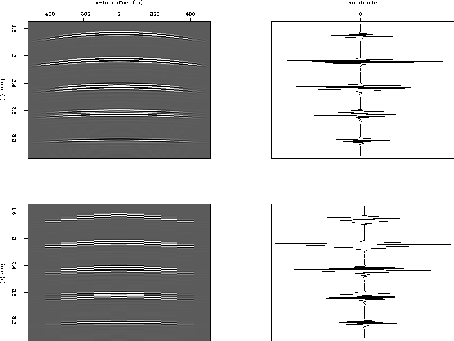
Figure 6 displays two PSMCGs with different sampling intervals and the corresponding stacked multiples. Unfortunately, a brutal summation in the sparsely sampled cross-line direction introduces a large amount of aliasing noise into the predicted multiple. The next section describes a method of avoiding such noise.
 |