

Next: Numerical Examples
Up: Sun: Multiple prediction
Previous: A Multiple Contribution Gather
The multiple prediction proposal discussed in the preceding section suggests
that we can estimate 3-D multiples without trace interpolation.
However, as Figure 6 shows, the other problem--aliasing
noise--has to be dealt with carefully if there is no missing-streamer
interpolation.
Like any other Kirchhoff-style operation, anti-aliasing is an important
issue in multiple prediction. This issue deserves even more attention
in three dimensions, since the cross-line sampling is more sparse than
the in-line sampling.
The 3-D estimation of a multiple trace is achieved by stacking a 3-D MCG.
As discussed in the preceding section, we can safely stack the 3-D MCG
into a 2-D PSMCG along the in-line direction. In the cross-line direction,
we must sample the PSMCG more densely to avoid the aliasing noise.
Therefore, I propose interpolating the PSMCG directly and then stack it
into a multiple trace.
We can interpolate the aliased data in either the F-X
Spitz (1991) or the T-X domain Claerbout (1992).
I have chosen the time-space domain multi-scale prediction-error filter
(MSPEF) theory discussed
in Section 8.4 of Claerbout (1992) to interpolate the PSMCG.
The basic idea of the theory is that large objects often resemble
small objects. Supposing that we have input data with alternate missing
traces, we can estimate a PEF with the following shape:
|  |
(1) |
Then we can make the filter smaller by throwing away the zeros (represented
by dots) in filter (1) to get
|  |
(2) |
which has the same dip characteristics as filter (1).
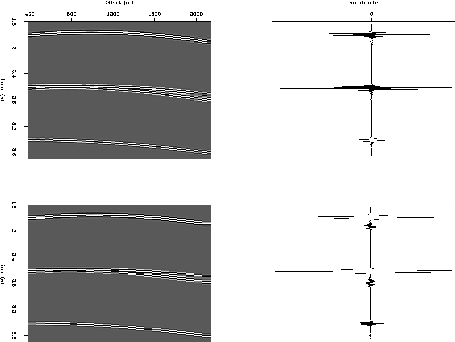
Figure 7 shows two PSMCGs containing crossing events,
before and after interpolating the alternative missing traces and the
corresponding stacking results. The aliasing noise has decreased significantly
after trace interpolation.
mcg-interp
Figure 7 Top: a densely sampled ( =25m) PSMCG and its stacking result. Bottom: a sparsely sampled (
 =50m) PSMCG and its stacking result. The aliasing noise has been greatly decreased after the trace interval is halved from 50m to 25m.


Next: Numerical Examples
Up: Sun: Multiple prediction
Previous: A Multiple Contribution Gather
Stanford Exploration Project
4/20/1999


