Numerical Examples

Combining the multiple prediction and the PSMCG interpolation, we get a new, practical multiple prediction scheme beyond two dimensions. In this section, two 3-D synthetic datasets with similar acquisition geometries are used to evaluate the new scheme. The corresponding model and acquisition parameters appear in Tables 1 and 2.

$$^\circ ^\circ$$ Model Layer velocity (km/s)

A (0.0,5.0,10.0) (0.0, 0.0, 0.0) (1.5, 2.0, 2.5)

B (0.0,5.0,10.0) (0.0, -5.0, 5.0) (1.5, 2.0, 2.5)

Table 1: Model parameters of Models A and B

$$\Delta_{\rm source} \Delta_{\rm receiver} \Delta_{\rm streamer}$$ Model

A 20 20 100

B 20 20 50

Table 2: Acquisition parameters of Models A and B

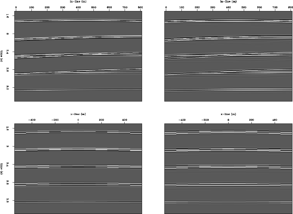
Model A is designed so that the shotline and streamers are deployed along the in-line dip direction. Therefore, there is no approximation error in our approach. With 11 streamers covering from -500m to +500m and a 100m streamer interval in the cross-line direction, this is a wide azimuth survey.

For a given shot location, Figure 8 shows the ideal multiple gather and the predicted one. Each 3-D MCG cube in this example is first stacked along the in-line direction into a 2-D PSMCG containing at most 11 traces sampled at intervals of 100m. The 2-D PSMCG is then interpolated in the cross-line direction to be sampled at 25m intervals. The interpolated PSMCG is further stacked into a trace.

 

wa2d-mult
Figure 8 An in-line dip model. Left: the ideal multiple reflection. Right: the estimated multiple reflection.

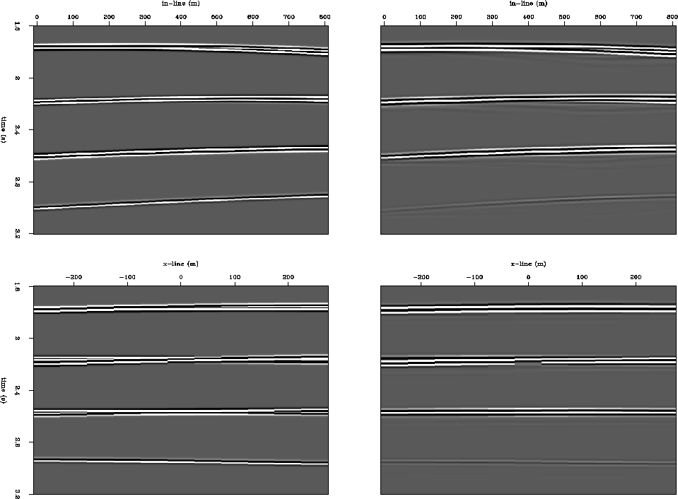
Model B is a relatively narrow azimuth survey that still contains 11 streamers covering from -250m to +250m at 50m streamer intervals in the cross-line direction. The bottom two reflectors in the model have the opposite cross-line angles, which inevitably introduce approximation error into the estimation. However, as shown in Figure 9, as long as the cross-line dips have no dominant direction, the error can possibly be compensated for in the subtraction step.

 

na3d-mult
Figure 9 A mixing dip model. Left: the ideal multiple reflection. Right: the estimated multiple reflection.