Signal and noise separation

We assume that the data vector $\bold d$ is composed of the signal and noise components $\bold s$ and $\bold n$: 

$$\bold{d = s + n}\;.$$ (5)

If both the signal and noise prediction-error filters S and N are known, then the signal can be extracted from the data by solving the following system by the least squares method:

$$\begin{eqnarray} 0 & \approx & \bold N \bold n = \bold N ( \bold d - \bold s)\;; \\ 0 & \approx & \epsilon \bold S \bold s\;,\end{eqnarray}$$ (6) (7)

where $\epsilon$ is a scalar scaling coefficient, reflecting the presumed signal-to-noise ration Claerbout (1999).

The formal solution of system (6-7) has the form of a projection filter :  

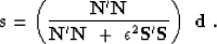$$\bold s = \left( \bold N' \bold N \over \bold N' \bold N \ + \ \epsilon^2 \bold S'\bold S \right) \ \bold d\;.$$ (8)

Analogously, the signal vector is expressed as  

$$\bold n = \bold d - \bold s = \left( \epsilon^2 \bold S' ... ...\bold N \ + \ \epsilon^2 \bold S'\bold S \right) \ \bold d\;.$$ (9)

In 1-D or F-X setting, one can accomplish the division in formulas (8) and (9) directly by spectral factorization and inverse recursive filtering Soubaras (1994, 1995). A similar approach can be applied in the case of T-X or F-XY filtering with the help of the helix transform Claerbout (1998); Ozdemir et al. (1999) or by solving system  (6-7) directly with an iterative method Abma (1995).

Claerbout's approach, implemented in the examples of GEE Claerbout (1999), is to estimate the signal and noise PEFs S and N from the data $\bold d$ by specifying different shape templates for these two filters. The filter estimates can be iteratively refined after the initial signal and noise separation. In some examples, such as those shown in this paper, the signal and noise templates are not easily separated. When the signal template behaves as an extension of the noise template so that the shape of S completely embeds the shape of N, our estimate of S serves as a predictor of both signal and noise. We might as well consider it as D, the prediction-error filter for the data.

Spitz (1999) argues that the data PEF D can be regarded as the convolution of the signal and noise PEFs S and N.

This assertion suggests the following algorithm:

1.

Estimate D and N.

2.

Estimate S by deconvolving (polynomial division) D by N.

3.

Solve the least-square system (6-7).

To avoid the division step, we suggest a simple modification of Spitz's algorithm, which results from multiplying both equations in system (6-7) by the noise filtering operator $\bold{N}$. The resulting system has the form

$$\begin{eqnarray} 0 & \approx & \bold N^2 \bold n = \bold N^2 ( \bold d - \bold ... ...x & \epsilon \bold N \bold S \bold s = \epsilon \bold D \bold s\;.\end{eqnarray}$$ (10) (11)

The modified algorithm is

1.

Estimate D and N.

2.

Convolve N with itself.

3.

Solve the least-square system (10-11).

The formal least-squares solution of system (10-11) is  

$$\bold s = \left( \bold {N' N' N N} \over \bold {N' N' N... ... N N} \ + \ \epsilon^2 \bold {N' S' S N} \right) \ \bold d\;.$$ (12)

Comparing (12) with (8), we can see that both the numerator and the denominator in the two expressions differ by the same multiplier $\bold{N' N}$. This multiplication should not effect the result of projection filtering.

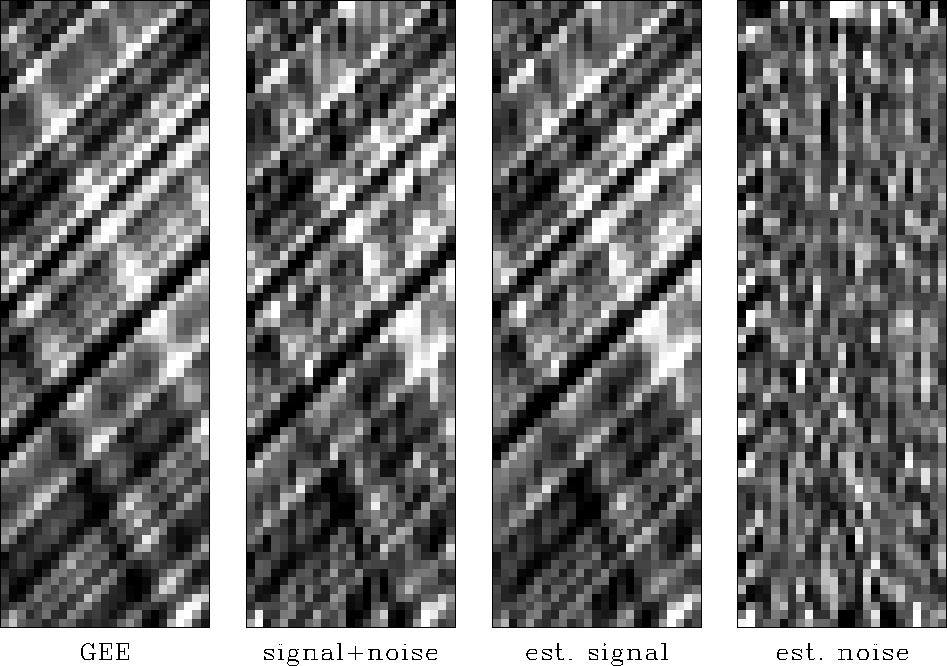
Figure 1 shows a simple example of signal and noise separation taken from GEE Claerbout (1999). The signal consists of two crossing plane waves with random amplitudes, and the noise is spatially random. The data and noise T-X prediction-error filters were estimated from the same data by applying different filter templates. The template for D is

  a a
  a a
  a a
1 a a
a a a
a a a
a a a

where the a symbol represents adjustable coefficients. The data filter shape has three columns, which allows it to predict two plane waves with different slopes. The noise filter N has only one column. Its template is

1
a
a
a

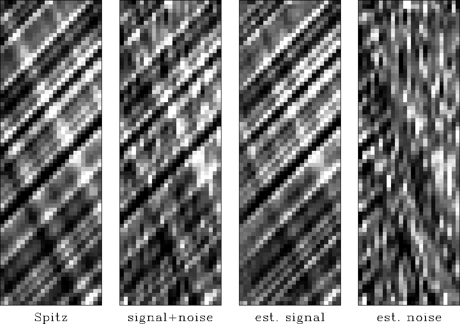
The noise PEF can estimate the temporal spectrum but would fail to capture the signal predictability in the space direction. Figure 2 shows the result of applying the modified Spitz method according to equations  (10-11). Comparing figures 1 and 2, we can see that using a modified system of equations brings a slightly modified result with more noise in the signal but more signal in the noise. It is as if $\epsilon$ has changed, and indeed this could be the principal effect of neglecting the denominator in equation (3).

 

signoi90
Figure 1 Signal and noise separation with the original GEE method. The input signal is on the left. Next is that signal with random noise added. Next are the estimated signal and the estimated noise.

 

signoi
Figure 2 Signal and noise separation with the modified Spitz method. The input signal is on the left. Next is that signal with random noise added. Next are the estimated signal and the estimated noise.

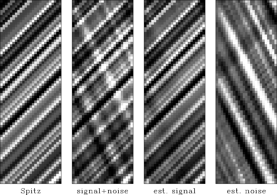
To illustrate a significantly different result using the Spitz insight we examine the new situation shown in Figures 3 and 4. The wave with the positive slope is considered to be regular noise; the other wave is signal. The noise PEF N was estimated from the data by restricting the filter shape so that it could predict only positive slopes. The corresponding template is

  a 
1 a

The data PEF template is

  a a
  a a
1 a a
a a a
a a a

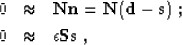
Using the data PEF as a substitute for the signal PEF produces a poor result, shown in Figure 3. We see a part of the signal sneaking into the noise estimate. Using the modified Spitz method, we obtain a clean separation of the plane waves (Figure 4).

 

planes90
Figure 3 Plane wave separation with the GEE method. The input signal is on the left. Next is that signal with noise added. Next are the estimated signal and the estimated noise.

 

planes
Figure 4 Plane wave separation with the modified Spitz method. The input signal is on the left. Next is that signal with noise added. Next are the estimated signal and the estimated noise.

Clapp and Brown (1999, 2000) and Brown et al. (1999) show applications of the least-squares signal-noise separation to multiple and ground-roll elimination.