 |
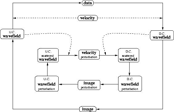
Figure 1 The chart of wave-equation migration velocity analysis technique. D.C. is a label for objects involved in the downward continuation branch, while U.C. is a label for the similar objects of the upward-continuation branch.
The imaging process described in the preceding paragraph requires that we make an assumption about the slowness model. We label this slowness the background model; therefore, the wavefield and image generated using this model are also naturally labeled as the background wavefield and image.
 |
Wave-equation modeling, the adjoint of migration, proceeds by upward-continuing the data from the highest depth and by adding contributions at every depth level. Eventually, we reach the surface and reconstruct the wavefield at the surface, which is equivalent, but not identical, to the recorded data.
A perturbation in the slowness model, excited by the background wavefield, generates a scattered wavefield. Like the background wavefield, this is downward continued, creating a wavefield perturbation, and is imaged, creating an image perturbation. In practice, we can either compute the background wavefield at the same time we compute the scattered wavefield, or we can compute and store it before, one frequency at a time.
As for the background, the adjoint process takes us from the image perturbation to an upward-continued wavefield from which we can derive at every depth level a scattered wavefield and, furthermore, a slowness perturbation.
This is the core theoretical result of the wave-equation migration velocity analysis technique: we can relate a perturbation in the slowness model to a perturbation in the migrated image. This enables us to improve the slowness model at the same time we improve the migrated image. This observation formally materializes a well-known concept: migration and velocity analysis are fundamentally related and inseparable from each other Gray (1998). This concept is not particular to our method, although the power of WEMVA lies in that it formally eliminates the distinction between velocity analysis and migration and aims at one single goal of image improvement.
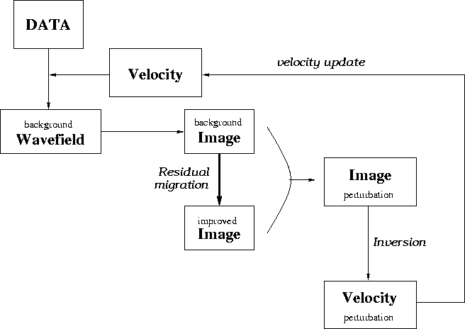
Our previous publication Biondi and Sava (1999) established the theoretical framework of the method. We have presented the mathematical foundations of the method and a few simple experiments. Here we go one step further and present a complete example starting with the data at the surface and ending with an improved slowness model. Figure 2 shows a flowchart of our method, that consists of the following major loop:
|
flow
Figure 2 A flowchart of wave-equation migration and WEMVA. |  |