Extension to 3-D

To construct $\bf T_{}$ we must derive a relationship between dt and $\bf \Delta s$. We will begin by defining two different slownesses: focusing and mapping slowness. The focusing slowness is the slowness that best focuses the data. The mapping slowness is the slowness that correctly positions the data.

Starting with mapping slowness s_m in terms of x,y, and z, we can transform into tau space through

$$\begin{eqnarray} \tau(z,x,y) &=& \int_0^z 2 s_m(z',x,y) dz' \nonumber \ x' &=& x \ y' &=& y, \nonumber\end{eqnarray}$$ (5)

where $\tau$ is the two-way vertical traveltime, x' is our new x coordinate, and y' is our new y coordinate. Using the chain rule we can derive the relationship between the derivatives of our coordinates,

$$\begin{eqnarray} \frac{\partial t}{\partial z} &=& \frac{\partial t}{\partial \t... ...tial \tau} \int_0^z \frac{\partial}{\partial y} 2s_m(z',x,y) dz' .\end{eqnarray}$$ (6) (7) (8)

We can simplify the above relations by defining two $\sigma$ quantities, one in the x-direction, $\sigma_x$, and one in the y-direction, $\sigma_y$,

$$\begin{eqnarray} \sigma_x(z,x,y) &=& \int_0^z \frac{\partial}{\partial x} 2s_m(z... ...z,x,y) &=& \int_0^z \frac{\partial}{\partial y} 2s_m(z',x,y) dz' .\end{eqnarray}$$ (9) (10)

Taking the derivative of both sides of the transform of (5) we can obtain a relation for dz, dx, and dy,

$$\begin{eqnarray} dz &=& \frac{d \tau}{2 s_m } -\frac{ \sigma_x dx'}{2 s_m} - \frac{\sigma_y dy '}{2 s_m} \ dx &=& dx' \ dy &=& dy' .\end{eqnarray}$$ (11) (12) (13)

To obtain our tomography operator in 3-D we begin by defining the traveltime along a single ray segment (where quantities measured along the ray segment are indicated by ) in tau space using equations (11-13),

$$\widetilde{dt} = \sqrt{ \left(\widetilde{S_f} \widetilde{dx'... ...ilde{dx'}- \widetilde{\sigma_y} \widetilde{dy'} }{2}\right)^2}$$ (14)

We can then take the derivative with respect to the focusing slowness s_f,

$$\begin{eqnarray} \frac{ d (\widetilde{dt})} {d S_f} = \frac{ \widetilde{S_f} \l... ..._f} + \widetilde{dy'} {d\widetilde{\sigma_y} \over ds_f} . \right)\end{eqnarray}$$ (15)

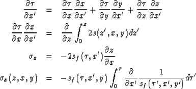
We new have an expression in terms of ${d\widetilde{S_f} \over ds_f}$, ${d\widetilde{\sigma_x} \over ds_f}$, and ${d\widetilde{\sigma_y} \over ds_f}$.To get an expression in terms of just $\frac{d\widetilde{S_f}} {ds_f}$we start by taking the partial derivative of $\tau$ with respect to x',

$$\begin{eqnarray} \frac{\partial \tau}{\partial x'} &=& \frac{\partial \tau}{\pa... ...rtial}{\partial x'} \frac{1}{ s_f(\tau',x',y')} d \tau' \nonumber \end{eqnarray}$$ (16)

and similarly

$$\sigma_y(z,x,y) =- s_f(\tau, x,y') \int_0^\tau \frac{\partial}{\partial y'} \frac{1}{ s_f(\tau',x',y')} d \tau' .$$ (17)

We then take the derivative with respect to s_f and evaluate at the ray segment,

$$\begin{eqnarray} \frac{\partial \widetilde{\sigma_x}}{\partial s_f} &=& {\wideti... ...al^2 s_f(\tau',x',y') }{\partial y' \partial s_f} \partial \tau' .\end{eqnarray}$$ (18) (19)

As a result we now have a linear relation between $\bf \Delta t$ and S_f in the tau domain.