B-splines

B-splines represent a particular example of a convolutional basis. Because of their compact support and other attractive numerical properties, B-splines are a good choice of the basis set for the forward interpolation problem and related signal processing problems Unser (1999). According to Thévenaz et al. (2000), they exhibit superior performance for any given order of accuracy in comparison with other methods of similar efficiency.

B-splines of the order 0 and 1 coincide with the nearest neighbor and linear interpolants () and () respectively. B-splines $\beta^n(x)$ of a higher order n can be defined by a repetitive convolution of the zeroth-order spline $\beta^0(x)$ (the box function) with itself:  

$$\beta^n(x) = \underbrace{\beta^0(x) \ast \cdots \ast \beta^0(x)}_{(n+1)\quad \mbox{times}}\;.$$ (68)

There is also the explicit expression  

$$\beta^n(x) = \frac{1}{n!}\,\sum_{k=0}^{n+1} C_k^{n+1} (-1)^k (x + \frac{n+1}{2} - k)_{+}^n\;,$$ (69)

which can be proved by induction. Here C_kⁿ⁺¹ are the binomial coefficients, and the function x₊ is defined as follows:  

$$x_{+} = \left\{\begin{array} {lcr} x, & \mbox{for} & x \gt 0 \\ 0, & \mbox{otherwise} &\end{array}\right.$$ (70)

As follows from formula (), the most commonly used cubic B-spline $\beta^3(x)$ has the expression  

$$\beta^3(x) = \left\{\begin{array} {lcr} \displaystyle \left... ...vert x\vert \geq 1 \\ 0, & \mbox{elsewhere} &\end{array}\right.$$ (71)

The corresponding discrete filter $\beta^3(n)$ is a centered 3-point filter with coefficients 1/6, 2/3, and 1/6. According to the traditional method, deconvolution with this filter is performed as a tridiagonal matrix inversion de Boor (1978). One can, however, accomplish the same task more efficiently by spectral factorization and recursive filtering Unser et al. (1993). The recursive filtering approach generalizes straightforwardly to B-splines of higher orders.

Both the support length and the smoothness of B-splines increase with the order. In the limit, B-splines converge to the Gaussian function. Figures  and  show the third- and seventh-order splines $\beta^3(x)$ and $\beta^7(x)$, respectively, and their continuous spectra.

 

splint3
Figure 13 Third-order B-spline $\beta^3(x)$ (left) and its spectrum (right).

 

splint7
Figure 14 Seventh-order B-spline $\beta^7(x)$ (left) and its spectrum (right).

It is important to realize the difference between B-splines and the corresponding interpolants W(x,n), which are sometimes called cardinal splines . An explicit computation of the cardinal splines is impractical, because they have infinitely long support. Typically, they are constructed implicitly by the two-step interpolation method outlined above. The cardinal splines of orders 3 and 7 and their spectra are shown in Figures  and . As B-splines converge to the Gaussian function, the corresponding interpolants rapidly converge to the sinc function (). Good convergence is achieved with the help of the implicitly-generated long support, which results from recursive filtering at the first step of the interpolation procedure.

 

crdint3
Figure 15 Effective third-order B-spline interpolant (left) and its spectrum (right).

 

crdint7
Figure 16 Effective seventh-order B-spline interpolant (left) and its spectrum (right).

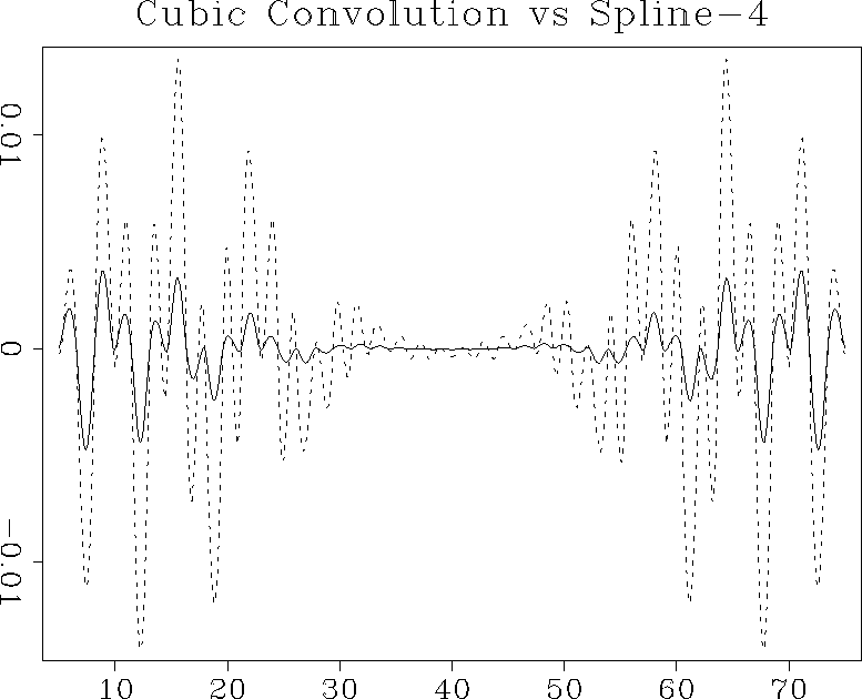
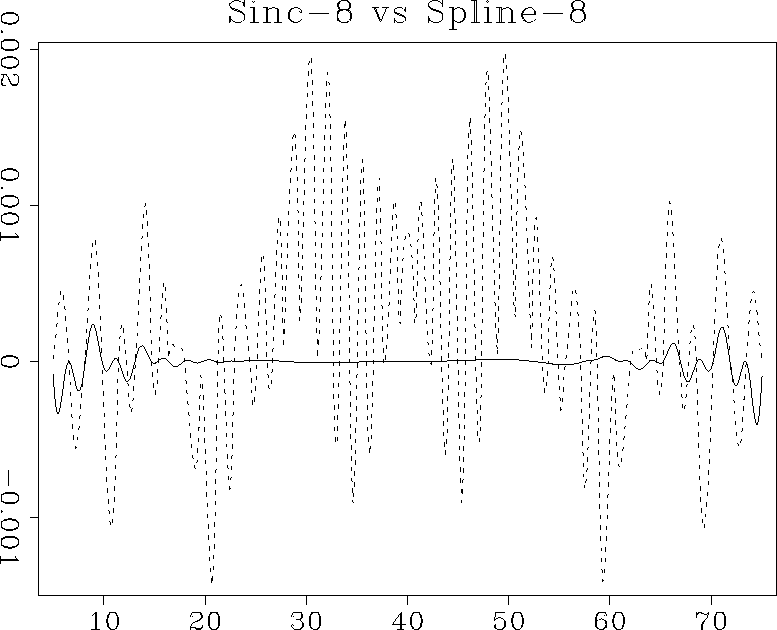
In practice, the recursive filtering step adds only marginally to the total interpolation cost. Therefore, an n-th order B-spline interpolation is comparable in cost with any other method that uses an (n+1)-point interpolant. The comparison in accuracy usually turns out in favor of B-splines. Figures  and  compare interpolation errors of B-splines and other similar-cost methods on the example from Figure .

 

cubspl Figure 17 Interpolation error of the cubic-convolution interpolant (dashed line) compared to that of the third-order B-spline (solid line).

 

kaispl Figure 18 Interpolation error of the 8-point windowed sinc interpolant (dashed line) compared to that of the seventh-order B-spline (solid line).

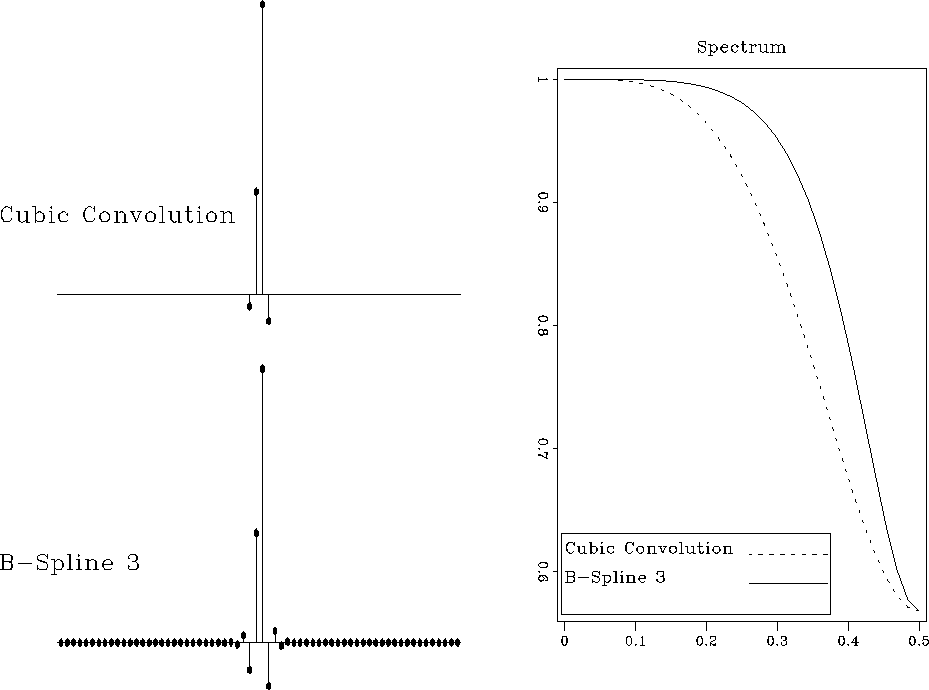
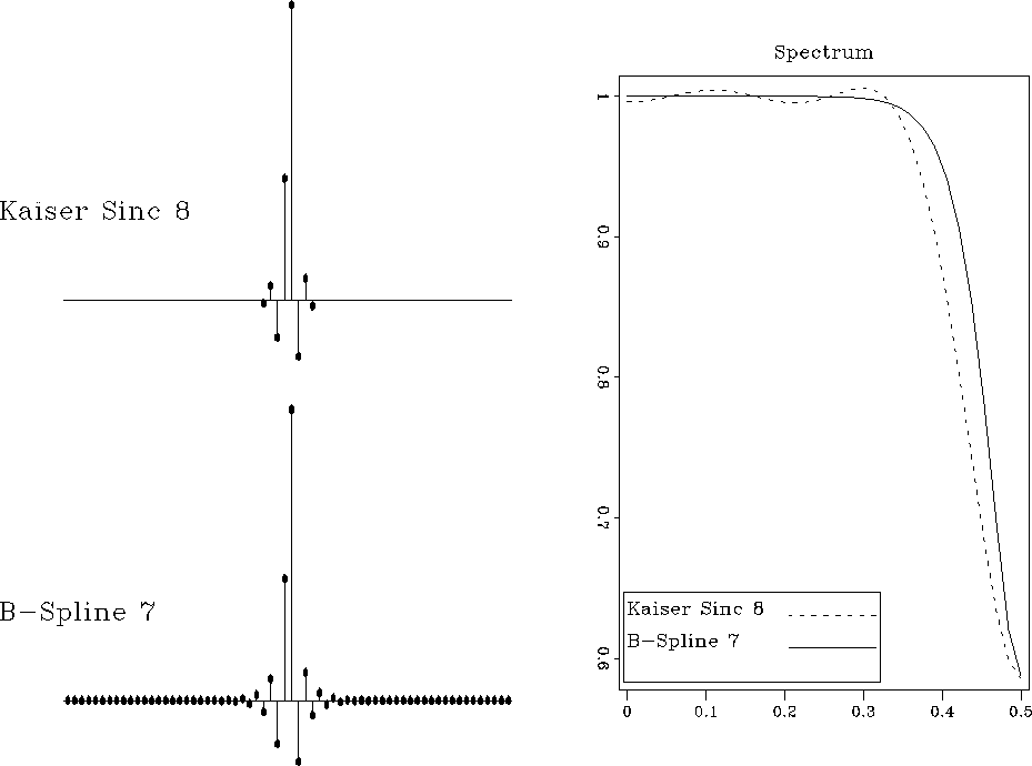
Similarly to the comparison in Figures  and , we can also compare the discrete responses of B-spline interpolation with those of other methods. The right plots in Figures  and  show that the discrete spectra of the effective B-spline interpolants are genuinely flat at low frequencies and wider than those of the competitive methods. Although the B-spline responses are infinitely long because of the recursive filtering step, they exhibit a fast amplitude decay.

 

speccubspl Figure 19 Discrete interpolation responses of cubic convolution and third-order B-spline interpolants (left) and their discrete spectra (right) for x=0.7.

 

speckaispl Figure 20 Discrete interpolation responses of 8-point windowed sinc and seventh-order B-spline interpolants (left) and their discrete spectra (right) for x=0.7.