Analytical solution for calculating time shifts

Another possible solution would be to solve the following equation to find the absolute time (t(x,y)) that minimizes (Fomel, 2002, personal communication)  

$$J(t) = \int \int \left[ \left( p_x(t,x,y)-\frac{\partial t}{... ...(t,x,y)-\frac{\partial t}{\partial y}\right)^2 \right] \,dx\,dy$$ (11)

where p_x is the dip in the x direction and p_y is the dip in the y direction.

Although this is for one horizon, it will be useful to solve this equation for all horizons simultaneously. This would allow the problem to be regularized and its solution to be truly global. In particular, it would no longer be necessary to iterate to remove residual structure in cases of the dip changing with time.

The Euler-Lagrange equation is used in calculus of variations Farlow (1993) to find a function (t) that will minimize a functional (J). It is analogous to the calculus expression for finding x to minimize the function f(x) in:  

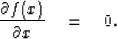$$\frac{\partial f(x)}{\partial x} \quad= \quad 0.$$ (12)

The Euler-Lagrange equation is applied to equation (11) to find (a simplified 2-D development is shown in Appendix A):  

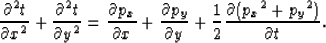$$\frac{\partial^2 t}{\partial x^2} + \frac{\partial^2 t}{\par... ... y} + \frac{1}{2} \frac{\partial({p_x}^2+{p_y}^2)}{\partial t}.$$ (13)

Figure is a 2-D example summarizing this flattening process for a single horizon. The 2-D version of equation (13) is:  

$$\frac{\partial^2 t}{\partial x^2} = \frac{\partial p_x}{\partial x}+ \frac{1}{2} \frac{\partial{p_x}^2}{\partial t}.$$ (14)

 

1horiz
Figure 7 (a) A 2-D cartoon image of a horizon to be flattened. (b) A 2-D image of the dip field showing only dip values along the horizon. (c) The output time field showing where the horizon will be mapped. (d) The calculated time shift values of the time field.

Figure a is a cartoon image of the horizon to be flattened. Figure b shows the dip field of that horizon. Figure c is the output time field. In this case, we are looping over the output field. Each value in Figure c contains time values of where to sample the data in order to flatten it. Figure d shows the time shift values from the output time field for this horizon.

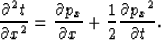
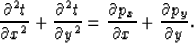
Equation (13) is non-linear and therefore tricky to solve because dip functions,p_x and p_y, are dependent on the unknown, t, and the last term is taking a derivative with respect to the unknown, t.

Incidentally, dropping the last term from equation 13, the equation can be simplified to:  

$$\frac{\partial^2 t}{\partial x^2} + \frac{\partial^2 t}{\par... ...ac{\partial p_x}{\partial x}+ \frac{\partial p_y}{\partial y} .$$ (15)

This is another way of writing equation (3), except that here the dip is a function of the output, t. Repeated applications of this equation partially accommodates for the dropping of the last term.