


![[*]](http://sepwww.stanford.edu/latex2html/cross_ref_motif.gif) . Two characteristics
distinguish this medium from the continuous 1-D medium whose
behavior is described by the wave equation. First, energy is localized
in discrete points in space. Second, the internal forces are dissociated
from mass, which implies that traction is not continuous
since each mass is considered as a rigid body.
. Two characteristics
distinguish this medium from the continuous 1-D medium whose
behavior is described by the wave equation. First, energy is localized
in discrete points in space. Second, the internal forces are dissociated
from mass, which implies that traction is not continuous
since each mass is considered as a rigid body.
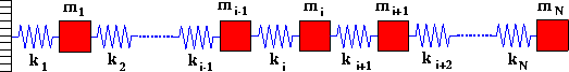 |

Newton's law applied to the ith mass of Figure
leads to the following equation:
| |
(1) |
The system of equations defined by equation (1) with i=1,N can be expressed as
| |
(2) |
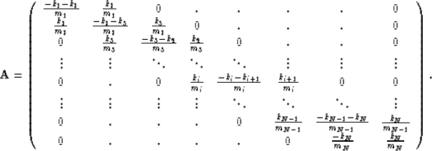
This is a second-order system of N ordinary differential equations
in time for the N unknown functions ![]() . To find the
solution, the pair of initial conditions u(0) and
. To find the
solution, the pair of initial conditions u(0) and ![]() must be specified. For the continuous case, the wave equation has also a
second-order space differentiation, and thus requires two boundary conditions.
Here, these two conditions correspond to the first and last equations.
must be specified. For the continuous case, the wave equation has also a
second-order space differentiation, and thus requires two boundary conditions.
Here, these two conditions correspond to the first and last equations.
Fourier transforming equation (2) over time results in
| |
(3) |
Let ![]() be the matrix formed by the eigenvectors
be the matrix formed by the eigenvectors ![]() of
of
![]() and
and ![]() the diagonal matrix with the respective
eigenvalues. If
the diagonal matrix with the respective
eigenvalues. If ![]() is Hermitian, then the set of eigenvectors
is Hermitian, then the set of eigenvectors
![]() form a complete orthonormal basis for
form a complete orthonormal basis for ![]() .If the masses are identical
.If the masses are identical ![]() is real-symmetric and the
general solution
is real-symmetric and the
general solution ![]() is given by
is given by
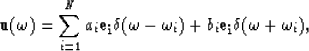 |
(4) |
| |
(5) |
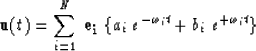
Applying the initial conditions to equation (5) and recalling
that ![]() is orthonormal, we find the equation for the unknowns c
and d:
is orthonormal, we find the equation for the unknowns c
and d:
![]()
Substituting this result in equation (5) and in the equivalent
relation for ![]() results in
results in
| |
(6) |
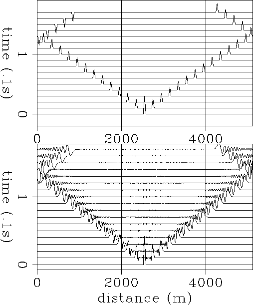
Figure compares the exact, analytical solution of the wave equation
(-a) with the discrete-model solution (-b) from
equation (6). The initial conditions are ![]() and
and ![]() . There are two important
differences between the two cases: the dispersive character of the
propagating wave-packet in the discrete case, and the continuing irradiation
of energy from the impulsive source position, which is also only present
in the discrete case. In both cases the
spectrum is characterized by a discrete set of frequencies because the
model is spatially bounded, but, while in the continuous case the set
is infinite, in the discrete case only N components are present which
implies an upper frequency limit.
. There are two important
differences between the two cases: the dispersive character of the
propagating wave-packet in the discrete case, and the continuing irradiation
of energy from the impulsive source position, which is also only present
in the discrete case. In both cases the
spectrum is characterized by a discrete set of frequencies because the
model is spatially bounded, but, while in the continuous case the set
is infinite, in the discrete case only N components are present which
implies an upper frequency limit.
 |


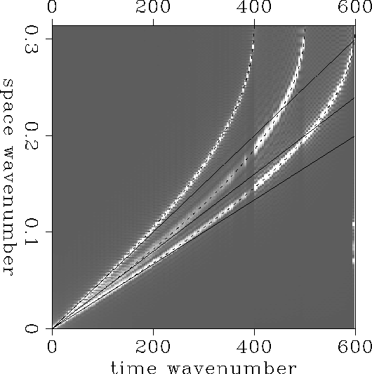
A clear picture of the dispersion process can be obtained from
the eigenvalue-eigenvector structure. Each eigenvector ![]() corresponds to a spatial harmonic associated with the eigenfrequency
corresponds to a spatial harmonic associated with the eigenfrequency
![]() . If we Fourier transform these eigenvectors and rescale the
vertical axis by
. If we Fourier transform these eigenvectors and rescale the
vertical axis by ![]() , the resulting matrix
, the resulting matrix ![]() will represent
the spatial spectra of the model. To get the dispersion relation it is
necessary to stretch the horizontal axis using the eigenfrequencies
will represent
the spatial spectra of the model. To get the dispersion relation it is
necessary to stretch the horizontal axis using the eigenfrequencies ![]() , so that the spectra will be a function of
, so that the spectra will be a function of ![]() instead of i.
Figure compares the
instead of i.
Figure compares the ![]() spectrum obtained with this
process with the dispersion relation predicted by the wave equation
(continuous line) and with the function
spectrum obtained with this
process with the dispersion relation predicted by the wave equation
(continuous line) and with the function ![]() (dashed line) predicted by the
discretized wave equation (Claerbout, 1985). The dispersion relation shown
in this figure was generated from the eigen-spectrum of a three-layer model.
The relation between the maximum spatial and temporal frequencies
(dashed line) predicted by the
discretized wave equation (Claerbout, 1985). The dispersion relation shown
in this figure was generated from the eigen-spectrum of a three-layer model.
The relation between the maximum spatial and temporal frequencies
![]() is valid not only for the discrete case
but also for the continuous case. The meaning of such relation is
that the minimum time interval for transmission of energy between
adjacent points is equal to half the fundamental period
is valid not only for the discrete case
but also for the continuous case. The meaning of such relation is
that the minimum time interval for transmission of energy between
adjacent points is equal to half the fundamental period ![]() .
The difference is that
.
The difference is that ![]() for the continuous case while
for the continuous case while
![]() for a discrete system with distance
for a discrete system with distance ![]() between masses.
between masses.
The intrinsically dispersive character of wave propagation in a discrete medium can also be related to the entropic behavior of a discrete system. In a continuous medium, the constraints imposed by the continuity of stresses and displacements represent a hampering of the process of the increasing of entropy, while in a discrete system, the extra degree of freedom (no continuity constraints) allows the system to evolve into less ordered states of movement.
 |