


| |
(9) |
Jacobs (1982) compared the implementation of three different forms of
equation (9), in a pre-stack profile migration in the
![]() domain:
domain:
![\begin{eqnarraystar}
R_1 & = & \int \; \phi^r \; [\phi^s]^{\ast} \; d \omega, \\...
...i^s]^{\ast} \over \mid \phi^s \mid^2 +
\epsilon} \; d \omega.\end{eqnarraystar}](img30.gif) |
||
The implementation of the P-P reflectivity imaging-condition stated in equation 2 with the correlation criterion (9) uses the following definitions:
![]()
![]()
![]()
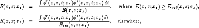 |
||
| (10) |
| |
(11) |
In the above equations, Ecut(x,z;xs) is a smooth function that should
approximate a fraction of the inverse of the spherical divergence.
Equation (10) gives the correct estimation of the reflection
coefficient in the regions well illuminated by the source
(![]() ) and a damped estimation in the dim regions.
) and a damped estimation in the dim regions.
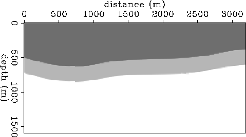 |


Figures ![[*]](http://sepwww.stanford.edu/latex2html/cross_ref_motif.gif) and show two images obtained
with equations (10 and 11). The difference between these
figures is that a smooth background model was used in the extrapolation step
for Figure and the original discontinuous model was used
in the extrapolation step for Figure . The source is located
at position 800 meters and the receivers extends from 980 meters to 2480 meters.
and show two images obtained
with equations (10 and 11). The difference between these
figures is that a smooth background model was used in the extrapolation step
for Figure and the original discontinuous model was used
in the extrapolation step for Figure . The source is located
at position 800 meters and the receivers extends from 980 meters to 2480 meters.
 |
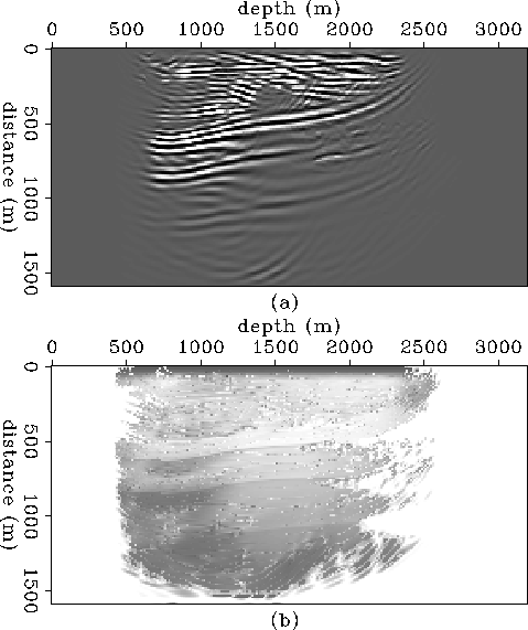 |
Using a smooth background velocity avoids the contamination of
the image by false reflectors originated by reflections in the
extrapolation stage. In addition, the two wavefields involved in
the migration correspond to unmixed modes (incident and reflected).
One disadvantage is that transmission/conversion losses in the
interfaces above the target are not compensated for in the extrapolation
step. Another disadvantage is the loss in resolution caused by the higher
dispersion in the wavefield extrapolation when a smooth background model
is used![[*]](http://sepwww.stanford.edu/latex2html/foot_motif.gif) .
.
When a non-smoothed background model is used in the extrapolation step the
upward propagating modeled field and the downward propagating recorded field
can be left out of the imaging computation, but the secondary reflections
generated by them will generate false events in the final imaging. Also,
at each interface (where the imaging computation is relevant) the two
wavefields involved in the migration correspond to a superposition of several
modes (incident, reflected, transmitted and converted) resulting in a
contradictory application of the imaging principle.
Nevertheless, there are two positive aspects in the use of a discontinuous
model. First, the transmission/conversion losses are correctly compensated
(at least for the incident wavefield ![]() .), and second, the small
dispersion results in a superior resolution.
.), and second, the small
dispersion results in a superior resolution.
Figure shows the images obtained for the other modes
using the correlation criterion implementation of equations (4),
(5), and (6). In this figure, both -a and
-b refer to the PS reflectivity but while -a
was obtained using the true model, -b was generated using a
smoothed model for P velocities and discontinuous (true) for S velocities.
The other two images, which correspond to SP (-c) and SS
(-d) modes, were also obtained using the true velocity model.
All the mode-converted images obtained with a smoothed velocity model were
completely unreliable because the mode-conversion dynamics of smooth models
is notably different from the mode-conversion dynamics of discontinuous media.
Even when the discontinuous model is used we can see false events which
are not related to the generation of multiples as in the PP case.
Although the ocean floor interface should be absent from all the converted-mode images we can see from the figure that it is actually present in all of them. The reason is that the reverse-propagating P wavefield is partially converted to S in the liquid-solid boundary and the correlation of this converted wavefield with the modeled wavefield (which is also also partially converted to S) produces the false images. These false images of the ocean floor are actually deeper than the PP images because they are formed below the boundary. There are however some positive aspects in these converted-mode images. As expected the regions where the propagation-direction of the wavefield is nearly normal to the interface are not imaged, while some strong reflections can be observed at regions where the incidence angle is large.
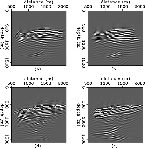 |
. (a) P-S reflectivity
using the unsmoothed velocity model. (b) P-S reflectivity using a smoothed
P velocity and the unsmoothed S velocity. (c) S-P reflectivity using the
unsmoothed velocity model. (d) S-S reflectivity using the unsmoothed
velocity model.