


Given the premise that conventional sonic logs measure vertical travel time in the formation, we make the assumption that the elastic properties of the layer are isotropic. This may or may not be the case, but could only be determined with more additional measurements. An rms velocity calculation following Dix, uses that vertical velocity to come up with an NMO velocity. This velocity is isotropic (unless extended to anisotropy as shown by Dellinger and Muir (1993)). The §+M averaging works with hybrid matrices of stiffness and compliance. Thus it requires P wave and S wave velocities and density in a layer to be known. If we again make the assumption of an isotropic layer, these three parameters determine the elastic properties uniquely. However, using the §+M average, the resulting average layer, may or may not be isotropic. This is in contrast to the conventional Dix average and will manifest itself in differences between vertical velocity (depth mapping) and Move-out velocity (NMO velocity).
Nowadays, P and S wave sonics, and density measurements are more commonly recorded than in the past, where only P wave sonics and density were available. If we do not have a shear wave log available, we would need to estimate one from other auxiliary information. In the examples in this paper I assumed a constant pressure/shear wave velocity ratio. Which is clearly in error in the target zone since the reservoir will have a different Poisson ratio than the embedding medium.
Some well logs include a dipmeter measurement, giving an estimate of the spatial orientation of a layer. The dip of a plane layer can be one more possible parameter in the §+M average, It has the effect that the coordinate system in which the average is carried out is rotated appropriately. Since the §+M average is based on the elastic properties, it can readily incorporate any information that might be possibly measured in the future, like velocities at different propagation angles and orientations.
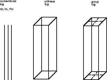 |

Fig. 4 illustrates the ``elastic log'' used during averaging. Having a reasonable method of scaling well log information up to surface seismic measurements may help in constraining stacking velocities during velocity analysis at points close to a seismic line. it may also help in estimating velocities for depth mapping (in general focusing and depth mapping velocities are not identical). In this paper I base my analysis on stacking velocities, but the application to focusing and depth mapping is straight forward extension.