AN EXAMPLE OF A COMPLEX GEOLOGICAL MODEL

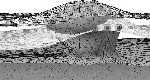
Figure 3 represents a model of a salt dome that pierces the two interfaces situated above the salt layer.

 

diapcut
Figure 3 Diapir model used to build the 3-D grid.

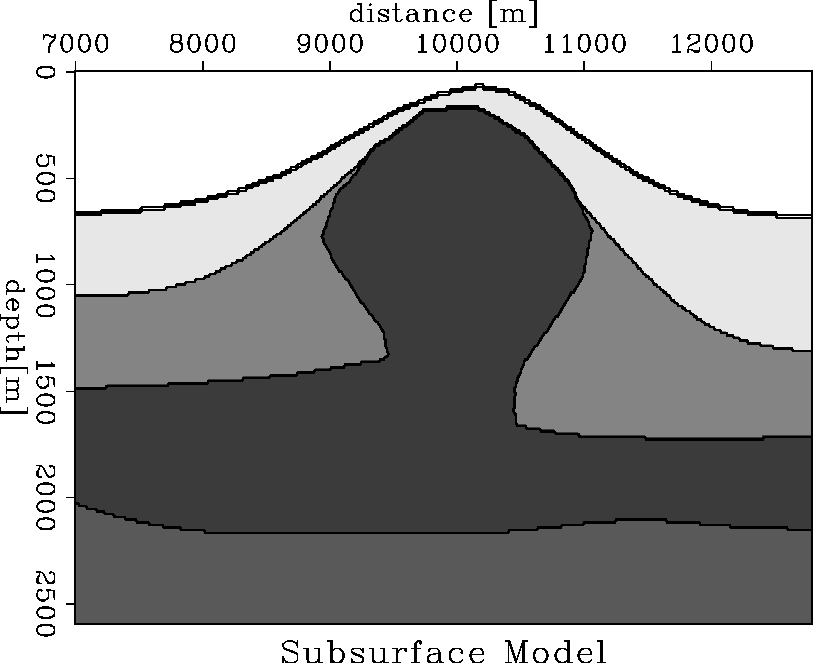
A model with 200 gridpoints in depth and 464 gridpoints in horizontal distance is written out of GOCAD and fed into a finite-difference modeling program Karrenbach (1992). Figure 4 shows the subsurface model. It consists of homogeneous sedimentary layers that are uplifted and intruded by a salt body, a classic diapir. We use a pressure source in an acoustic medium and collect the z-component of the displacement on the free surface of the model. 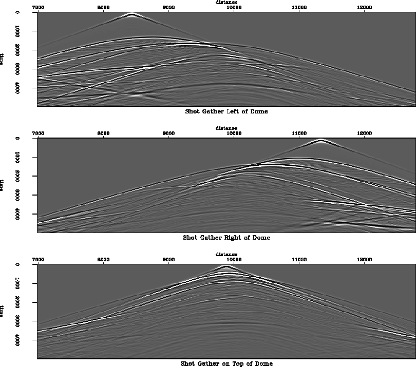The wavelet is a derivative of a Gaussian function with a fundamental frequency of 40Hz. Figure 5 shows z-component seismograms collected left, on top and right of the diapir.

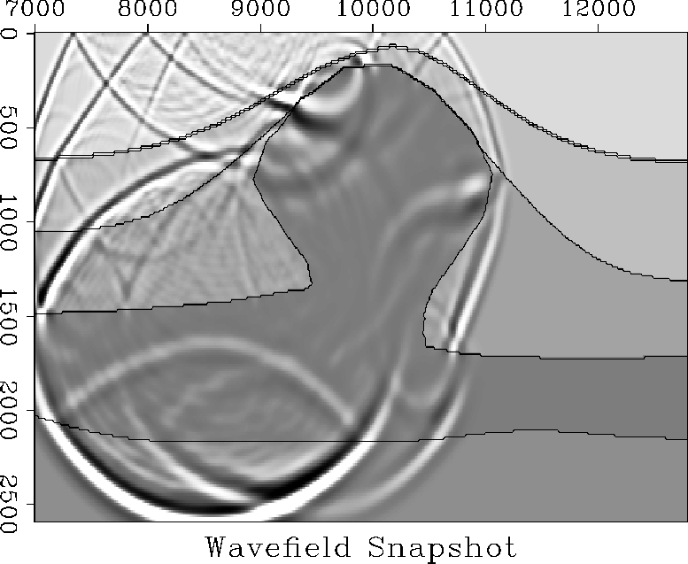
As explained previously, the gridding quality depends partly on the smoothness of the model interfaces. We can see some diffractions caused by stair-stepping of the first layer interface in Figure 4. During the wave propagation, the corners of those steps will act as diffraction points. In Figure 6, the snapshot of the z-component of the wave field, those outward propagating diffraction circles are clearly visible. On the seismograms, those diffraction points manifest themselves as hyperbolae suspended from the main reflection hyperbola. To watch the movie of those snapshots press the button at the end of the figure caption in Figure 6.

 

diap
Figure 4 Gridded output of the diapir model. Press button to sweep through the 3-D model cube.

 

zseis
Figure 5 Three shot gathers collected over the diapir model.

 

over.left
Figure 6 Snapshot of the wavefield at elapsed time 1.5 sec. Press button for a complete movie.