Interpolation in Stolt migration

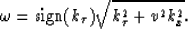
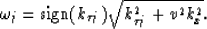
Depending on the method used to transform the field $P(\omega,k_x)$ into the interpolated field $P(\omega(k_{\tau},k_x),k_x)$, different artifacts can be introduced in the migrated image (Harlan, 1982; Ronen, 1982). One way to eliminate the interpolation and avoid artifacts in the migrated image is to perform a slow Fourier transform in time with irregular values in $\omega$, but regular in $k_{\tau}$: 

$$M(\tau,k_x)=\int dk_{\tau} e^{i k_{\tau} \tau} J(k_{\tau},k_... ...i{\rm sign}(k_{\tau})\sqrt{k_{\tau}^2 + v^2 k_x^2}t } P(t,k_x),$$ (5)

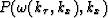
where $\omega$ was replaced by  

$$\omega ={\rm sign}(k_{\tau})\sqrt{k_{\tau}^2 + v^2 k_x^2}.$$ (6)

Actually such an algorithm can be very appealing when implemented on a parallel computer (Blondel, 1993) due to the high degree of parallelism, and can run faster than the sequence of FFT followed by interpolation. The mapping function from $(\omega,k_x)$ space to $(k_{\tau},k_x)$ can be any anisotropic dispersion relation. Dellinger et al. (1990) and Ecker and Muir (1993) show examples of anisotropic migration operators by modifying the dispersion relation (2).

By comparing the standard Stolt migration with the slow Fourier transform Stolt migration, we can deduce an interpolation scheme that, when used in connection with the standard algorithm, will be equivalent to the slower but more correct one. In matrix format, we can write the slow Fourier FFT for a single wavenumber k_x as:  

$$M(k_{\tau};k_x)= \left[ \begin{array} {c} P(\omega_1;k_x) ... ...\ P(t_2;k_x) \\ \vdots \\ P(t_n;k_x) \\ \end{array}\right].$$ (7)

The variable $\omega$ is not evenly sampled as required by the FFT. Each $\omega_j$ corresponds to an evenly sampled value of $k_{\tau}$according to equation (6)

$$\omega_j ={\rm sign}(k_{\tau j})\sqrt{k_{\tau j}^2 + v^2 k_x^2}.$$

The ones in the slow FT matrix represent zero values of time in the first column, i.e. t₁=0.

We can multiply the data by a unit matrix composed from a forward FFT and an inverse FFT before performing the slow FT

$$\left[ P(\omega_i;k_x) \right ] = \left[ SFT \right] \left[ FFT^{-1} \right] \left[ FFT \right] \left[ P(t_i;k_x) \right].$$ (8)

We observe that by combining the operations  

$$\left[ SFT \right] \left[ FFT^{-1} \right]$$ (9)

and calling it interpolation, we obtain the classic Stolt migration algorithm. What is left now is to identify exactly what our interpolation is doing.