


 |
(15) | |
| (16) |
The spatial tiling we have chosen gives us two independent locations for
storing density ![]() ,one atop the horizontal velocity u,
the other atop the vertical velocity v.
It may seem non physical to have one density
for vertical accelerations and another for horizontal ones,
but it is worth maintaining the two densities
as separate entities.
Waves arise from many physical paradigms besides the
acoustical one and some of these
may require that we maintain this possibility to introduce anisotropy.
Another way to introduce anisotropy in the present codes
is to have two compressibilities K in the pressure subroutine.
These extra parameters might also be helpful if
we were trying to improve the numerical representation
of the differential operators.
Subroutine velocity() uses
rhou(,) for
,one atop the horizontal velocity u,
the other atop the vertical velocity v.
It may seem non physical to have one density
for vertical accelerations and another for horizontal ones,
but it is worth maintaining the two densities
as separate entities.
Waves arise from many physical paradigms besides the
acoustical one and some of these
may require that we maintain this possibility to introduce anisotropy.
Another way to introduce anisotropy in the present codes
is to have two compressibilities K in the pressure subroutine.
These extra parameters might also be helpful if
we were trying to improve the numerical representation
of the differential operators.
Subroutine velocity() uses
rhou(,) for ![]() at u and
rhov(,) for
at u and
rhov(,) for ![]() at v.
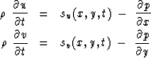
Equation (15) in discrete form
at v.
Equation (15) in discrete form
| |
(17) |
# Operator of momentum change from gradient of pressure
#
subroutine velocity( adj, add, rhou,rhov,  q,nx,ny,    r )
integer              adj, add,               nx,ny,       x, y,  p,   u,   v
real rhou(nx,ny), rhov(nx,ny), q(nx,ny,3), r(nx,ny,3)
call        adjnull( adj, add,             q,nx*ny*3,  r,nx*ny*3)
							        p=1; u=2; v=3
do x= 2, nx-1 {
do y= 2, ny-1 {
    if( adj == 0) {
	r(x,y,u)= r(x,y,u) + q(x,y,u) - ( q(x+1,y  ,p) - q(x,y,p)) * rhou(x,y)
	r(x,y,v)= r(x,y,v) + q(x,y,v) - ( q(x  ,y+1,p) - q(x,y,p)) * rhov(x,y)
	r(x,y,p)= r(x,y,p) + q(x,y,p)
    } else {
	q(x  ,y  ,u)= q(x  ,y  ,u) + r(x,y,u)
	q(x  ,y  ,p)= q(x  ,y  ,p) + r(x,y,u) * rhou(x,y) + r(x,y,p)
	q(x+1,y  ,p)= q(x+1,y  ,p) - r(x,y,u) * rhou(x,y)
	#
	q(x  ,y  ,v)= q(x  ,y  ,v) + r(x,y,v)
	q(x  ,y  ,p)= q(x  ,y  ,p) + r(x,y,v) * rhov(x,y)
	q(x  ,y+1,p)= q(x  ,y+1,p) - r(x,y,v) * rhov(x,y)
	}
    }}
return; end
This time we pass through the pressure unchanged so we also see an added pressure term in the adjoint.