TWO-STAGE LINEAR LEAST SQUARES

In Chapter and Chapter we filled empty bins by minimizing the energy output from the filtered mesh. In each case there was arbitrariness in the choice of the filter. Here we find and use the optimum filter, the PEF.

The first stage is that of the previous section, finding the optimal PEF while carefully avoiding using any regression equations that involve boundaries or missing data. For the second stage, we take the PEF as known and find values for the empty bins so that the power out of the prediction-error filter is minimized. To do this we find missing data with module mis2() .

This two-stage method avoids the nonlinear problem we would otherwise face if we included the fitting equations containing both free data values and free filter values. Presumably, after two stages of linear least squares we are close enough to the final solution that we could switch over to the full nonlinear setup described near the end of this chapter.

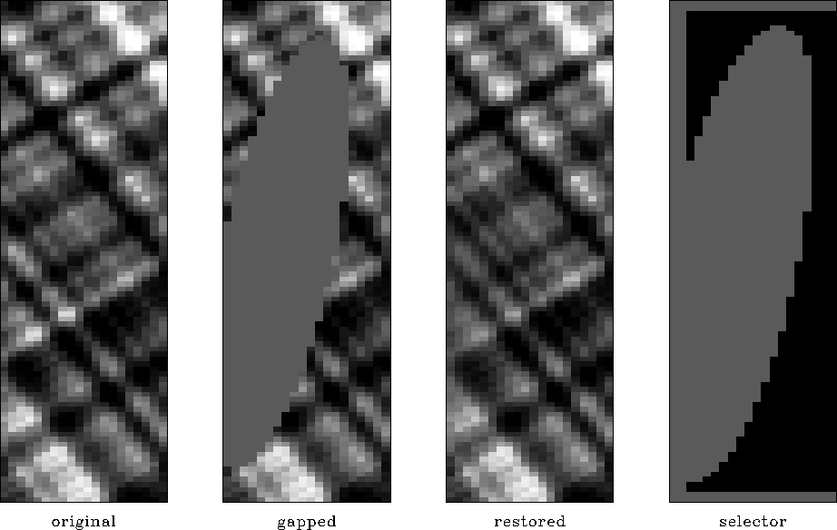
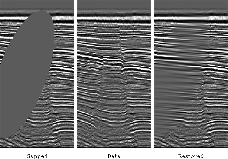
The synthetic data in Figure 14 is a superposition of two plane waves of different directions, each with a random (but low-passed) waveform. After punching a hole in the data, we find that the lost data is pleasingly restored, though a bit weak near the side boundary. This imperfection could result from the side-boundary behavior of the operator or from an insufficient number of missing-data iterations.

 

hole90
Figure 14 Original data (left), with a zeroed hole, restored, residual selector (right).

The residual selector in Figure 14 shows where the filter output has valid inputs. From it you can deduce the size and shape of the filter, namely that it matches up with Figure 10. The ellipsoidal hole in the residual selector is larger than that in the data because we lose regression equations not only at the hole, but where any part of the filter overlaps the hole.

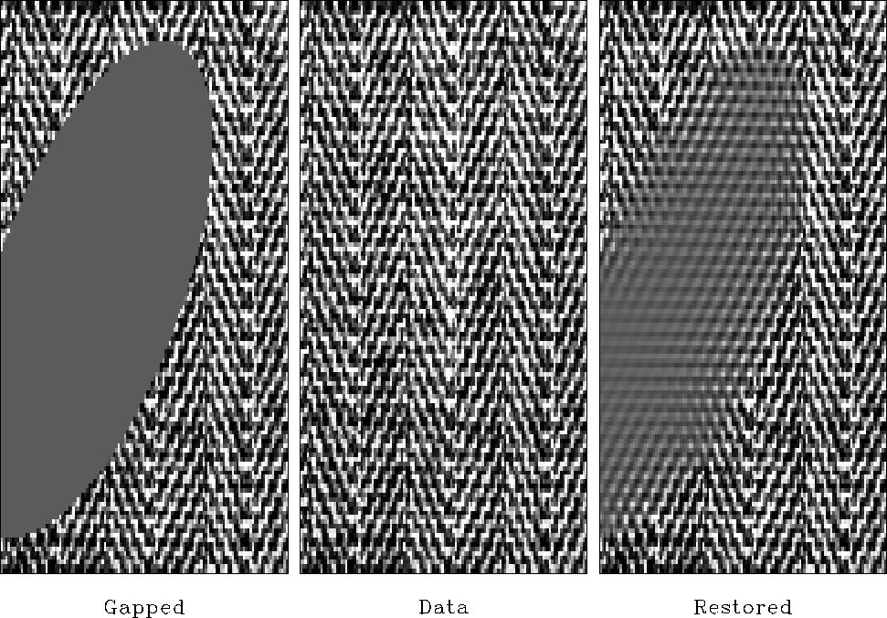
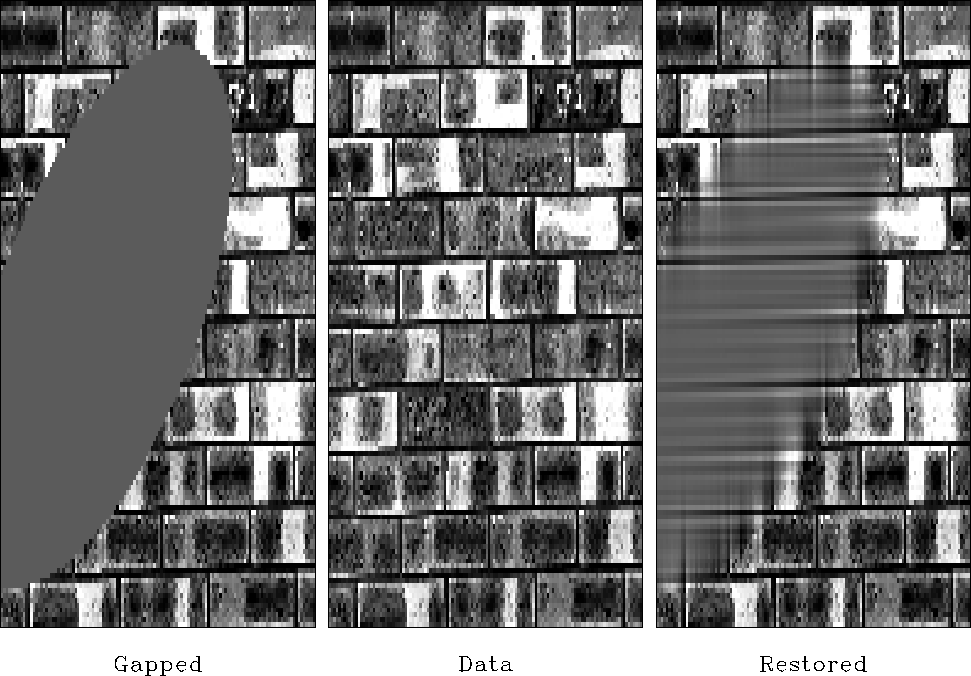
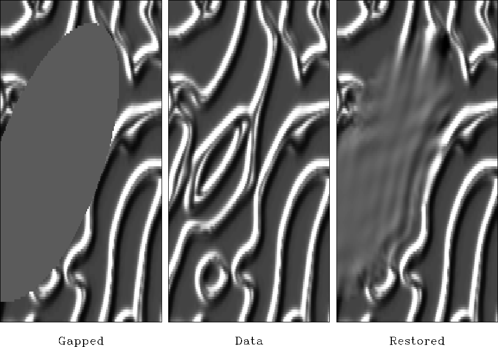
The results in Figure 14 are essentially perfect representing the fact that that synthetic example fits the conceptual model perfectly. Figures 15-18 show real data of various kinds.

 

herr-hole-fill
Figure 15 The herringbone texture is a patchwork of two textures. We notice that data missing from the hole tends to fill with the texture at the edge of the hole. The spine of the herring fish, however, is not modeled at all.

 

brick-hole-fill
Figure 16 The brick texture has a mortar part (both vertical and horizontal joins) and a brick surface part. These three parts enter the empty area but do not end where they should.

 

ridges-hole-fill
Figure 17 The theoretical model is a poor fit to the ridge data since the prediction must try to match ridges of all possible orientations. This data requires a broader theory which incorporates the possibility of nonstationarity (space variable slope).

 

WGstack-hole-fill
Figure 18 Filling the missing seismic data. The imaging process known as ``migration'' would suffer diffraction artifacts in the gapped data that it would not suffer on the restored data.