SYLVESTER'S MATRIX THEOREM

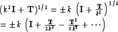
Sylvester's theorem provides a rapid way to calculate functions of a matrix. Some simple functions of a matrix of frequent occurrence are ${\bf A}^{-1}$ and ${\bf A}^N$ (for N large). Two more matrix functions which are very important in wave propagation are $e^{\bf A}$ and ${\bf A}^{1/2}$.Before going into the somewhat abstract proof of Sylvester's theorem, we will take up a numerical example. Consider the matrix  

$${\bf A} \eq \left[ \begin{array} {rr} 3 & -2 \\ 1 & 0 \end{array} \right]$$ (26)

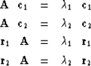
It will be necessary to have the column eigenvectors and the eigenvalues of this matrix; they are given by

$$\begin{eqnarray} \left[ \begin{array} {rr} 3 & -2 \\ 1 & 0 \end{array} \right]... ...ght] \eq 2\, \left[ \begin{array} {c} 2 \\ 1 \end{array} \right]\end{eqnarray}$$ (27) (28)

Since the matrix A is not symmetric, it has row eigenvectors which differ from the column vectors. These are

$$\begin{eqnarray} \left[-1 \quad 2\right] \, \left[ \begin{array} {rr} 3 & -2 \\... ... -2 \\ 1 & 0 \end{array} \right] &= & 2\, \left[1 \quad -1\right]\end{eqnarray}$$ (29) (30)

We may abbreviate equations (27) through (30) by

$$\begin{eqnarray} {\bf A} \ \ {\bf c}_1 &= & \lambda_1 \ \ {\bf c}_1 \nonumber \\... ..._1 \\ {\bf r}_2 \ \ {\bf A} &= & \lambda_2 \ \ {\bf r}_2 \nonumber\end{eqnarray}$$ (31)

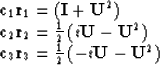
The reader will observe that r or c could be multiplied by an arbitrary scale factor and (31) would still be valid. The eigenvectors are said to be normalized if scale factors have been chosen so that ${\bf r}_1 \cdot {\bf c}_1 = 1$ and ${\bf r}_2 \cdot {\bf c}_2 =1$.It will be observed that ${\bf r}_2 \cdot {\bf c}_2 = 0$ and ${\bf r}_2 \cdot {\bf c}_1 = 0$,a general result to be established in the exercises.

Let us consider the behavior of the matrix ${\bf c}_1 {\bf r}_1$.

$${\bf c}_1 {\bf r}_1 \eq \left[ \begin{array} {c} 1 \\ 1 \... ... \left[ \begin{array} {cc} -1 & 2 \\ -1 & 2 \end{array} \right]$$

Any power of this matrix is the matrix itself, for example its square.

$$\left[ \begin{array} {cc} -1 & 2 \\ -1 & 2 \end{array} \righ... ... \left[ \begin{array} {cc} -1 & 2 \\ -1 & 2 \end{array} \right]$$

This property is called idempotence (Latin for self-power). It arises because $({\bf c}_1 {\bf r}_1) ({\bf c}_1 {\bf r}_1) = {\bf c}_1 ({\bf r}_1 \cdot {\bf c}_1)\, {\bf r}_1 = {\bf c}_1 {\bf r}_1$.The same thing is of course true of ${\bf c}_2 {\bf r}_2$. Now notice that the matrix ${\bf c}_1 {\bf r}_1$ is ``perpendicular'' to the matrix ${\bf c}_2 {\bf r}_2$, that is

$$\left[ \begin{array} {cc} 2 & -2 \\ 1 & -1 \end{array} \righ... ...q \left[ \begin{array} {cc} 0 & 0 \\ 0 & 0 \end{array} \right]$$

since ${\bf r}_2$ and ${\bf c}_2$ are perpendicular.

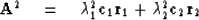
Sylvester's theorem says that any function f of the matrix A may be written

$$f({\bf A}) \eq f(\lambda_1) \, {\bf c}_1 {\bf r}_1 + f(\lambda_2) \, {\bf c}_2 {\bf r}_2$$

The simplest example is $f({\bf A}) = {\bf A}$

$$\begin{eqnarray} {\bf A} &= & \lambda_1 \, {\bf c}_1 {\bf r}_1 + \lambda_2 \, {... ... \eq \left[ \begin{array} {rr} 3 & -2 \\ 1 & 0 \end{array} \right]\end{eqnarray}$$ (32)

Another example is

$$A^2 \eq 1^2\, \left[ \begin{array} {cc} -1 & 2 \\ -1 & 2 \e... ... \left[ \begin{array} {rr} 7 & -6 \\ 3 & -2 \end{array} \right]$$

The inverse is

$$A^{-1} \eq 1^{-1}\, \left[ \begin{array} {cc} -1 & 2 \\ -1 ... ..., \left[ \begin{array} {rr} 0 & 2 \\ -1 & 3 \end{array} \right]$$

The identity matrix may be expanded in terms of the eigenvectors of the matrix A.

$$A^0 \eq {\bf I} \eq 1^0\, \left[ \begin{array} {cc} -1 & 2 ... ...eq \left[ \begin{array} {rr} 1 & 0 \\ 0 & 1 \end{array} \right]$$

Before illustrating some more complicated functions let us see what it takes to prove Sylvester's theorem. We will need one basic result which is in all the books on matrix theory, namely, that most matrices (see exercises) can be diagonalized. In terms of our $2 \times 2$ example this takes the form  

$$\left[ {{\bf r}_1 \over {\bf r}_2} \right] {\bf A}\, [{\bf c... ...array} {cc} \lambda_1 & 0 \\ 0 & \lambda_2 \end{array} \right]$$ (33)

where  

$$\left[ {{\bf r}_1 \over {\bf r}_2} \right] \, [{\bf c}_1 \mi... ...q \left[ \begin{array} {cc} 1 & 0 \\ 0 & 1 \end{array} \right]$$ (34)

Since a matrix commutes with its inverse, (34) implies  

$$[{\bf c}_1 \mid {\bf c}_2] \, \left[ {{\bf r}_1 \over {\bf r... ...q \left[ \begin{array} {cc} 1 & 0 \\ 0 & 1 \end{array} \right]$$ (35)

Postmultiply (33) by the row matrix and premultiply by the column matrix. Using (35), we get  

$${\bf A} \eq [{\bf c}_1 \mid {\bf c}_2] \left[ \begin{array}... ...\end{array} \right] \left[ {{\bf r}_1 \over {\bf r}_2} \right]$$ (36)

Equation (36) is (32) in disguise, as we can see by writing (36) as Now to get ${\bf A}^2$ we have

$${\bf A}^2 \eq (\lambda_1 {\bf c}_1 {\bf r}_1 + \lambda_2 {\b... ...(\lambda_1 {\bf c}_1 {\bf r}_1 + \lambda_2 {\bf c}_2 {\bf r}_2)$$

Using the orthonormality of ${\bf c}_1 {\bf r}_1$ and ${\bf c}_2 {\bf r}_2$this reduces to

$${\bf A}^2 \eq \lambda_1^2 {\bf c}_1 {\bf r}_1 + \lambda_2^2 {\bf c}_2 {\bf r}_2$$

It is clear how (36) can be used to prove Sylvester's theorem for any polynomial function of A. Clearly, there is nothing peculiar about $2 \times 2$ matrices either. This works for $n \times n$.Likewise, one may consider infinite series functions in A. Since almost any function can be made up of infinite series, we can consider also transcendental functions like sine, cosine, exponential.

Exponentials arise naturally as the solutions to differential equations. Consider the matrix differential equation  

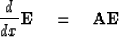$${d \over dx} {\bf E} \eq {\bf AE}$$ (37)

One may readily verify the power series solution

$${\bf E} \eq {\bf I} + {\bf A}x + {{\bf A}^2 x^2 \over 2!} + \cdots$$

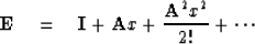
This is the power series definition of an exponential function. If the matrix A is one of that vast majority which can be diagonalized, then the exponential can be more simply expressed by Sylvester's theorem. For the numerical example we have been considering, we have

$${\bf E} \eq e^x \, \left[ \begin{array} {cc} -1 & 2 \\ -1 &... ... \left[ \begin{array} {cc} 2 & -2 \\ 1 & -1 \end{array} \right]$$

The exponential matrix is a solution to the differential equation (37) without regard to boundaries. It frequently happens that physics gives one a differential equation  

$${d \over dx} \, \left[ \begin{array} {c} y_1 \\ y_2 \end{a... ...f A}\, \left[ \begin{array} {c} y_1 \\ y_2 \end{array} \right]$$ (38)

Subject to two boundary conditions on either of y₁ or y₂ or a combination. One may verify that

$$\left[ \begin{array} {c} y_1 \\ y_2 \end{array} \right] \eq... ...}x} \, \left[ \begin{array} {c} k_1 \\ k_2 \end{array} \right]$$

is the solution to (38) for arbitrary constants k₁ and k₂. Boundary conditions are then used to determine the numerical values of k₁ and k₂. Note that k₁ and k₂ are just y₂ (x = 0) and y₂ (x = 0).

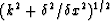
An interesting situation arises with the square root of a matrix. A $2 \times 2$ matrix like A will have four square roots because there are four possible combinations for choice of plus or minus signs on $\sqrt{\lambda_1}$ and $\sqrt{\lambda_2}$.In general, an $n \times n$ matrix has 2ⁿ square roots. An important application arises in a later chapter, where we will deal with the differential operator $(k^2 + \delta^2/\delta x^2)^{1/2}$.The square root of an operator is explained in very few books and few people even know what it means. The best way to visualize the square root of this differential operator is to relate it to the square root of the matrix M where

$${\bf M} \eq k^2 \, \left[ \begin{array} {ccccc} 1 & && & \\... ...-2 & 1 & \\ && 1 & -2 & 1 \\ & & & ? & ? \end{array} \right]$$

The right-hand matrix is a second difference approximation to a second partial derivative. Let us define

$${\bf M} \eq k^2 {\bf I} + {\bf T}$$

Clearly we wish to consider M generalized to a very large size so that the end effects may be minimized. In concept, we can make M as large as we like and for any size we can get $2^{\bf M}$ square roots. In practice there will be only two square roots of interest, one with the plus roots of all the eigenvalues and the other with all the minus roots. How can we find these ``principal value'' square roots? An important case of interest is where we can use the binomial theorem so that The result is justified by merely squaring the assumed square root. Alternatively, it may be justified by means of Sylvester's theorem. It should be noted that on squaring the assumed square root one utilizes the fact that I and T commute. We are led to the idea that the square root of the differential operator may be interpreted as

$$\left( k^2 + {\partial^2 \over \partial x^2} \right)^{1/2} \eq k + {1 \over 2k}\, {\partial^2 \over \partial x^2} + \cdots$$

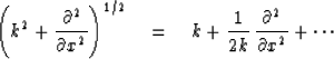
provided that k is not a function of x. If k is a function of x, the square root of the differential operator still has meaning but is not so simply computed with the binomial theorem.

EXERCISES:

1. Premultiply (31)b by ${\bf r}_1$ and postmultiply (31)c by ${\bf c}_2$,then subtract. Is $\lambda_1 \neq \lambda_2$a necessary condition for ${\bf r}_1$ and ${\bf c}_2$ to be perpendicular? Is it a sufficient condition?
2. Show the Cayley-Hamilton theorem, that is, if

   $$0 \eq f(\lambda) \eq {\rm det } ({\bf A} - \lambda {\bf I}) \eq p_0 + p_1 \lambda + p_2 \lambda^2 + \cdots p_n \lambda^n$$

   then

   $$f({\bf A}) \eq p_0 + p_1 {\bf A} + p_2 {\bf A}^2 + \cdots + p_n{\bf A}^n \eq 0$$

3. Verify that, for a general $2 \times 2$ matrix A, for which where $\lambda_1$ and $\lambda_2$ are eigenvalues of A. What is the general form for ${\bf c}_2 {\bf r}_2$?
4. For a symmetric matrix it can be shown that there is always a complete set of eigenvectors. A problem sometimes arises with nonsymmetric matrices. Study the matrix

   $$\left[ \begin{array} {rc} 1 & 1 - \epsilon^2 \\ -1 & 3 \end{array} \right]$$

   as $\epsilon \rightarrow 0$ to see why one eigenvector is lost. This is called a defective matrix. (This example is from T. R. Madden.)
5. A wide variety of wave-propagation problems in a stratified medium reduce to the equation

   $${d \over dx} \, \left[ \begin{array} {c} y_1 \\ y_2 \end{... ...] \, \left[ \begin{array} {c} y_1 \\ y_2 \end{array} \right]$$

   What is the x dependence of the solution when ab is positive? When ab is negative? Assume a and b are independent of x. Use Sylvester's theorem. What would it take to get a defective matrix? What are the solutions in the case of a defective matrix?
6. Consider a matrix of the form ${\bf I} + {\bf vv}^T$ where v is a column vector and ${\bf v}^T$ is its transpose. Find $({\bf I} + {\bf vv}^T)^{-1}$ in terms of a power series in ${\bf vv}^T$.[Note that $({\bf vv}^T)^n$ collapses to ${\bf vv}^T$ times a scaling factor, so the power series reduces considerably.]
7. The following ``cross-product'' matrix often arises in electrodynamics. Let ${\bf B} = (B_x, B_y, B_z)$

   $$U \eq {1 \over \sqrt{{\bf B} \cdot {\bf B}}} \, \left[ \beg... ... & B_y \\ B_z & 0 & -B_x \\ -B_y & B_x & 0 \end{array} \right]$$

   (a)

   Write out elements of ${\bf I} + {\bf U}^2$.

   (b)

   Show that ${\bf U} ({\bf I} + {\bf U}^2) =0$ or ${\bf U}^3 = -{\bf U}$.

   (c)

   Let ${\bf v}$ be an arbitrary vector. In what geometrical directions do Uv, ${\bf U}^2{\bf v}$, and $({\bf I} + {\bf U}^2) {\bf v}$ point?

   (d)

   What are the eigenvalues of U? [Hint:  Use part (b).]

   (e)

   Why cannot U be canceled from ${\bf U}^3 = -{\bf U}$?

   (f)

   Verify that the idempotent matrices of U are