MATRIX FILTERS, SPECTRA, AND FACTORING

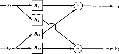
Two time series can be much more interesting than one because of the possibility of interactions between them. The general linear model for two series is depicted in Figure 1.

 

5-2 Figure 1 Two time series x1 and x2 input to a matrix of four filters illustrates the general linear model of multichannel filtering.

The filtering operation in the figure can be expressed as a matrix times vector operation, where the elements of the matrix and vectors are Z transform polynomials. That is,  

$$\left[ \begin{array} {c} Y_1 (Z) \\ Y_2 (Z) \end{array} \ri... ...left[ \begin{array} {c} X_1 (Z) \\ X_2 (Z) \end{array} \right]$$ (39)

One fact which is obvious but unfamiliar is that a matrix with polynomial elements is exactly the same thing as a polynomial with matrix coefficients. This is illustrated by the example:

$$\left[ \begin{array} {cc} 1 + Z + 2Z^2 & Z \\ 1 & 1 + Z^2 \... ...[ \begin{array} {cc} 2 & 0 \\ 0 & 1 \end{array} \right] \, Z^2$$

Now we can address ourselves to the inverse problem; given a filter B and the outputs Y how can we find the inputs X? The solution is analogous to that of single time series. Let us regard ${\bf B}(Z)$ as a matrix of polynomials. One knowns, for example, that the inverse of any $2 \times 2$ matrix

$$\left[ \begin{array} {cc} a & b \\ c & d \end{array} \right... ...ay} {cc} d & -b \\ -c & a \end{array} \right] \over {ad - bc}}$$

Consequently ${\bf Y} = {\bf BX}$ may be solved for X as ${\bf X} = {\bf B}^{-1} {\bf Y}$ where

$${\bf B}^{-1} \eq \left[ \begin{array} {rr} B_{22} (Z) & -B_... ...\right] \, {1 \over B_{11}(Z) B_{22}(Z) - B_{12}(Z) B_{21}(Z)}$$

The denominator is a scalar. We have treated scalar denominators before. If all the zeros lie outside the unit circle, we can use an ordinary power series for the inverse; otherwise, it is not minimum-phase and we use a Laurent series.

When one generalizes to many time series, the numerator matrix is the so-called adjoint matrix and the denominator is the determinant. The adjoint matrix can be formed without the use of any division operations. In other words, elements in the adjoint matrix are in the form of sums of products. For this reason, we may say that the criterion for a minimum-phase matrix wavelet is that the determinant of its Z transform has no zeros inside the unit circle.

Equation (39) is a useful description of Figure 1 in most applications. However in some applications (where the filter is an unknown to be determined), a transposed form of (39) is more useful. If b₁₂ was interchanged with b₂₁ in Figure 1, we could use the ``row data'' expression  

$$[Y_1 (Z) \quad Y_2 (Z)] \eq [X_1 (Z) \quad X_2 (Z)] \, \left[... ...ay} {cc} B_{11} & B_{12} \\ B_{21} & B_{22} \end{array} \right]$$ (40)

Now that we have generalized the concept of filtering from scalar-valued time series to vector-valued series, it is natural to generalize the idea of spectrum. For vector-valued time functions, the spectrum is a matrix called the spectral matrix and it is given by

$$\begin{eqnarray} {\bf R}(\omega) &= & \left[ \begin{array} {cc} r_{11} & r_{12} ... ...erline{Y}_2 Y_1 & \overline{Y}_2 Y_2 \end{array} \right] \nonumber\end{eqnarray}$$ (41)

It will be noticed that the vector times vector operation defining (41) is an ``outer product'' rather than the more usually occurring ``inner product.'' The diagonals of the spectral matrix R contain the usual auto-spectrum of each channel. Off-diagonals contain the cross spectrum. Because (41) is an outer product, the matrix is singular. Now, instead of taking $[Y_1 (Z) \ \ Y_2(Z)]$ to have a time function with a finite amount of energy, let us suppose the filter inputs to (40), namely (x₁ (t), x₂ (t)) are made up of random numbers, independently drawn from some time series and their spectral matrix is defined like (41) but taking an expectation (average over the ensemble). We have

$${\bf R} (\omega) \eq E \left[ \begin{array} {cc} \overline{Y}_1 \\ \overline{Y}_2 \end{array} \right] \, [Y_1 \ \ Y_2]$$

substituting from (40)

$${\bf R} (\omega) \eq E \left[ \begin{array} {cc} \overline{B... ... {B}_{11} & {B}_{12} \\ {B}_{21} & {B}_{22} \end{array} \right]$$

Now, grouping the ensemble summation with the random variables, we get  

$${\bf R} \eq \left[ \begin{array} {cc} \overline{B}_{11} & \o... ... {B}_{11} & {B}_{12} \\ {B}_{21} & {B}_{22} \end{array} \right]$$ (42)

Next, we explicitly introduce the assumption that the random numbers x₁ (t) are drawn independently of x₂ (t), thus $E(\overline{X}_2 (1/z) X_1 (z)) = 0$and the assumption that x_i(t) is white E[x_i (t) x_i (t + s)] = 0 is $s \neq 0$ and of unit variance E[x_i (t)²] = 1. Thus (42) becomes

$$\begin{eqnarray} {\bf R} &= & \left[ \begin{array} {cc} \overline{B}_{11} & \ov... ...cc} {B}_{11} & {B}_{12} \\ {B}_{21} & {B}_{22} \end{array} \right]\end{eqnarray}$$ (43)

Of course, in practice the spectral matrix must be estimated, say $\hat{\bf R}$, from finite samples of data. This means that ensemble summation must be simulated. If the ensembles sum in (42) is simulated by summation over one point (no summation), then (42) is a singular matrix like (41). As discussed earlier, the accuracy of the elements of the spectral matrix improves with the square root of the number of ensemble elements summed over.

Single-channel spectral factorization gives insight into numerous important problems in mathematical physics. We have seen that the concepts of filter and spectrum extend in quite a useful fashion to multichannel data. It was only natural that a great deal of effort should have gone to spectral factorization of multichannel data. This effort has been successful. However, in retrospect, from the point of view of computer modeling and interpretation of observed waves, it must be admitted that multichannel spectral factorization has not been especially useful. Nevertheless a brief summary of results will be given.

The root method. I extended the single-channel root method to the multichannel case. The method is even more cumbersome in the multichannel case. A most surprising thing about the solution is that it includes a much broader result: that a polynomial with matrix coefficients may be factored. For example,

$$\left[ \begin{array} {cc} 1 & 0 \\ 0 & 1 \end{array} \right]... ...left[ \begin{array} {rr} -4 & 4 \\ -58 & 28 \end{array} \right]$$

factors 6 ways to

The Toeplitz method. The only really practical method for finding an invertible matrix wavelet with a given spectrum is the multichannel Toeplitz method. The necessary algebra is developed in a later section on multichannel time series prediction.

The exp-log and Hilbert transform methods. A number of famous mathematicians including Norbert Wiener have worked on the problem from the point of view of extending the exp-log or the Hilbert transform method. The principal stumbling block is that exp(A + B) does not equal exp(A) exp(B) unless A and B happen to commute, that is, AB = BA. This is usually not the case. Although many difficult papers have appeared on the subject (some stating that they solved the problem), the author is unaware of anyone who ever wrote a computer program which works at fast Fourier transform speeds as does the single-channel Hilbert transform method.

EXERCISES:

1. Think up a matrix filter where the two outputs y₁(t) and y₂(t) are the same but for a scale factor. Clearly X cannot be recovered from Y. Show that the determinant of the filter vanishes. Find another example in which the determinant is zero at one frequency but nonzero elsewhere. Explain in the time domain in what sense the input cannot be recovered from the output.
2. Given a thermometer which measures temperature plus $\alpha$ times pressure and a pressure gage which measures pressure plus $\beta$ times the time rate of change of the temperature, find the matrix filter which converts the observed series to temperature and pressure. [HINT:  Use either the time derivative approximation 1 - Z or 2 (1 - Z)/(1 + Z).]
3. Let

   $${\bf B}(Z) \eq \left[ \begin{array} {cc} 1 & 0 \\ 3 & 2 \end... ...\, \left[ \begin{array} {cc} 2 & 1 \\ 0 & 0 \end{array} \right]$$

   Identify coefficients of powers of Z in ${\bf B}(Z) {\bf A}(Z) = {\bf I}$,to develop recursively the coefficients of ${\bf A}(Z) = [{\bf B}(Z)]^{-1}$.
4. Express the inverse of

   $$\left[ \begin{array} {cc} 1 + 2Z & Z \\ 3 & 2 \end{array} \right]$$

   in a Taylor or Laurent series as is necessary.
5. The determinant of a polynomial with matrix coefficients may be independent of Z. Applied to matrix filters, this may mean that an inverse filter may have only a finite number of powers in Z instead of the infinite series one always has with scalar filters. What is the most nontrivial example you can find?