ADAPTIVE FILTERS

An adaptive filter is one which changes with time to accommodate itself to changes in the time series being filtered. For example, suppose one were predicting one point ahead in a time series. One could take a lot of past data to design the filter; then one could apply the filter to present incoming data to predict future incoming data.

Below is a computer program to do the Burg algorithm. The program follows the notation of the text. The data X is a vector of dimension given to be LX. Choice of $LC \leq LX$ is a compromise between high resolution and high scatter. The density of points on the frequency axis, which is controlled by $N2048 \gg LX$, is chosen for plotting convenience and should be great enough to resolve narrow spectral lines.

       SUBROUTINE BURGC (LX,X,EP,EM,LC,C,A,N2048,S)
 C GIVEN A TIME SERIES X(1...LX) GET ITS LOG SPECTRUM S(1...N2048)
       DIMENSION X(LX),EP(LX),EM(LX),C(LC),A(LC),S(N2048)
       COMPLEX X,EP,EM,C,A,S,TOP,BOT,EPI,CONJG,CLOG
       DO 10 I=1,N2048
 10    S(I)=O.
       A(1)=1.
       DO 20 I=1,LX
       EM(I)=X(I)
 20    EP(I)=X(I)
       DO 60 J=2,LC
       TOP=0.
       BOT=0.
       DO 30 I=J,LX
       BOT=BOT+EP(I)*CONJG(EP(I))+EM(I-J+1)*CONJG(EM(I-J+1))
 30    TOP=TOP+EP(I)*CONJG(EM(I-J+1))
       C(J)=2*TOP/BOT
       DO 40 I=J,LX
       EPI=EP(I)
       EP(I)=EP(I)-C(J)*EM(I-J+1)
 40    EM(I-J+1)=EM(I-J+1)-CONJG(C(J))*EPI
       A(J)=0.
       DO 50 I=1,J
 50    S(I)=A(I)-C(J)*CONJG(A(J-I+1))
       DO 60 I=1,J
 60    A(I)=S(I)
       CALL FORK(N2048,S,+1.)
       DO 70 I=1,N2048
 70    S(I)=-CLOG(S(I))*2.
       RETURN
       END

As time goes on it might become desirable to recompute the filter on the basis of new data which have come in. How often should the filter be redesigned? In concept, there is no reason why it should not be recomputed very often, perhaps after each new data point arrives. In practice, this is usually prohibitively expensive. For a filter of length n it requires n multiplies and adds to apply the filter to get one new output point. To recompute the filter with Levinson recursion requires about n² multiply-adds. However, it is usually expected that the filter need only be changed by a very small amount when a new data point arrives. For that reason we will give the Widrow adaptive-filter algorithm which modifies the filter by means of only n arithmetic operations. Thus, a new filter is computed after each data point comes in.

For definiteness, consider a two-term prediction situation where e_t is the error in predicting a time series x_t from two of its past values  

$$e_t \eq x_t -bx_{t-1} - cx_{t-2}$$ (19)

The sum squared error in the prediction is  

$$E \eq \sum^{}_t {e_{t}}^2 \eq \sum^{}_t \; (x_t - bx_{t-1} -cx_{t-2})^2$$ (20)

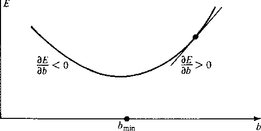
If the parameter b has been chosen correctly, one should find that $\partial \!E/ \partial b = 0$.However, if the nature of the time series x_t is changing with time, $\partial \!E/ \partial b$ may depart from zero when new data are included in the sum in (20). Since E is a positive quadratic function of b, if $\partial \!E/ \partial b$ has become positive, then b should be reduced. If $\partial \!E/ \partial b$ has become negative, then b should be augmented. See Figure 1.

 

7-2 Figure 1 The sign of the partial derivative tells whether $b \gt b_{\min}$ or $b < b_{\min}.$

From (20) we have  

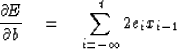$${\partial \!E \over \partial b} \eq \sum^t_{i = -\infty} 2e_{i}x_{i-1}$$ (21)

The change in $\partial \!E/ \partial b$ from the addition of the data point x_t is just -2e_tx_t-1; thus, we are motivated to modify b and c in the following way  

$$\left[ \begin{array} {c} b \\ c \end{array} \right] \lefta... ...eft[ \begin{array} {l} x_{t-1} \\ x_{t-2} \end{array} \right]$$ (22)

Here the number k scales the amount of the readjustment which we are willing to make to b and c in one time step. If k is chosen very small, the adjustment will take place very slowly. If k is chosen too large, the adjustment will overshoot the minimum; however one may hope that it will bounce back, perhaps again overshooting at the next step. The choice of k is dictated in part by the nature of the time series x_t under study.

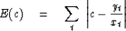
There are many variations on these same ideas. For example, we could use the L₁ norm and minimize something like  

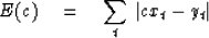$$E(c) \eq \sum^{}_t \:\vert cx_t - y_t\vert$$ (23)

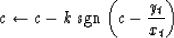
The resulting adaptation would be  

$$c \leftarrow c - kx_t \; \hbox{sgn} \;(cx_t - y_t)$$ (24)

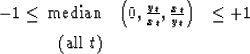
Equation (23) is of course the weighted median. An even more robust procedure is the uniformly weighted median  

$$E(c) \eq \sum^{}_t \; \left\vert c - {y_t \over x_t}\right\vert$$ (25)

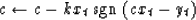
which leads to the adaptation  

$$c \leftarrow c - k \; \hbox{sgn} \left( c - {y_t \over x_t} \right)$$ (26)

which is identical to  

$$c \leftarrow c - k \; \hbox{sgn} \; (x_t) \; \hbox{sgn} \; (cx_t - y_t)$$ (27)

The examples (23) and (25) could be extended, in a manner like the Burg algorithm, to stationary series. Like (25) we could minimize  

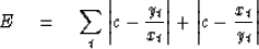$$E \eq \sum^{}_t \left\vert c - {y_t \over x_t}\right\vert + \left\vert c - {x_t \over y_t}\right\vert$$ (28)

This leads to a choice of c within the proper bounds because

$$\begin{eqnarray} -1 \leq\, \hbox{median} &\left( 0, {y_t \over x_t}, {x_t \over y_t}\right) & \leq + 1 \nonumber \\ * \hbox{(all}\;t) \nonumber\end{eqnarray}$$

EXERCISES:

1. If x_t has physical dimensions of volts, what should be the physical dimensions for k? If x_t has an rms value of 100 V and $\Delta t$,the sampling interval, is 1 ms, what numerical value of k will allow the Widrow filter to adapt to new conditions in about a second?
2. Consider the time series $x_t = (\ldots, 1, 1, 1, 1, -4, 1, 1, 1, 1, -4, 1, 1, 1, 1, -4, \ldots)$.Consider self-prediction of the form x_t+1 = cx_t. What are the results of least-squares prediction? What are the results of L₁ norm prediction of data weighted and uniformly weighted types?