BURG SPECTRAL ESTIMATION

The uncertainty principle says that if a time function contains most of its energy in the time-span $\Delta t$, then its Fourier transform contains most of its energy in a bandwidth $\Delta f \geq 1/\Delta t$. This is not the same as saying that if we have a sample of a stationary time series of length $\Delta t$,the best frequency resolution we can hope to attain will be $\Delta f = 1/\Delta t$.The difference lies in the difference between assuming a function is zero outside the interval $\Delta t$ in which it is given and in assuming that it continues ``in a sensible way" outside the given interval. If the data sample can be continued ``in a sensible way" some distance beyond the interval in which it is given, then the frequency resolution $\Delta f$ may be considerably smaller than $1/\Delta t$.A finer resolution depends upon the predictability of the data off the ends of the sample. If one has a segment of a stationary series which is short compared to the autocorrelation of the stationary series, then the spectral estimation procedure of John P. Burg will be radically better than any truncated Fourier transform method. This comes about in physical problems when one is dealing with resonances which have decay times that are long compared to the observation time or when one is looking at a function of space where each point in space represents another instrument.

If a spectrum R(Z) is estimated by $\bar{X}(1/Z)X(Z)$ where X(Z) is a polynomial made up from N + 1 known data points, then the coefficients of R(Z) are computed by  

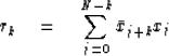$$r_k \eq \sum^{N - k}_{j = 0} \bar{x}_{j+k}x_j$$ (8)

Notice that r₀ is calculated from N + 1 terms, r₁ from N terms, etc. If N is not large enough, this will have an undesirable biasing effect. The biasing is removed if the r_k are computed instead by the formula  

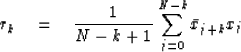$$r_k \eq {1 \over N - k + 1} \sum^{N-k}_{j = 0} \bar{x}_{j+k} x_j$$ (9)

The trouble with using (9) is that data samples can easily be found for which r_k will not be a valid autocorrelation function. For example, the spectrum will not be positive at all frequencies, the solution to Toeplitz equations may blow up, etc.

Burg's approach avoids the end-effect problems of (8) and the possibility of impossible results from (9). Instead of estimating the autocorrelation r_k directly from the data he estimates a minimum-phase prediction-error filter directly from the data. The output of a prediction-error filter has a white spectrum. (If it did not, then the color could be used to improve prediction.) Since the spectrum of the output is the spectrum of the input times the spectrum of the filter, the spectrum of the input may be estimated as the inverse of the spectrum of the prediction-error filter. As we have seen, narrow spectral peaks are far more easily represented by a denominator than by a numerator.

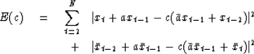
Let the given segment of data be denoted by $x_0, x_1, \ldots, x_n$.Then a two-term prediction-error filter (1,a) of the time series x_t is given by the choice of a which minimizes  

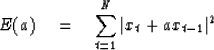$$E(a) \eq \sum^N_{t = 1} \vert x_t + ax_{t-1}\vert^2$$ (10)

Unfortunately, consideration of a few examples shows that there exist time series [like (1,2)] for which |a| may turn out to be greater than unity. This is unacceptable because the prediction-error filter is not minimum-phase, the spectrum is not positive, etc. Recall that a prediction-error filter defined in the previous section depends only on the autocorrelation of the data and not the data per se. This means that the same filter is computed from both a time series and from the (complex-conjugate) time-reversed time series. This suggests that the error of forward prediction (10) be augmented by the error of backward prediction. That is  

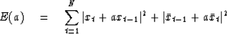$$E(a) \eq \sum^N_{t=1} \vert x_t + ax_{t-1}\vert^2 + \vert\bar{x}_{t-1} + a\bar{x}_t\vert^2$$ (11)

We will later establish that the minimization of (11) always leads to an |a| less than unity. The power spectral estimate associated with this value of a is $R = 1/[(1 + \bar{a}/Z)(1 + aZ)]$.The value of $\Delta f$ may be very small if a turns out very close to the unit circle.

A natural extension of (11) to filters with more terms would seem to be to minimize  

$$E(a_1,a_2) \eq \sum^N_{t=2} \vert x_t + a_{1}x_{t-1} + a_{2}... ...+ \vert\bar{x}_{t-2} + a_1 \bar{x}_{t-1} + a_2 \bar{x}_t\vert^2$$ (12)

Unfortunately, Burg discovered time series for which the computed filter A(Z) = 1 + a₁ Z + a₂ Z² was not minimum-phase. If A(Z) is not minimum-phase, then $R = 1/[\bar{A}(1/Z)A(Z)]$ is not a satisfactory spectral estimate because R(Z) is to be evaluated on the unit circle and 1/A(Z) would not be convergent there.

Burg noted that the Levinson recursion always gives minimum-phase filters. In the Levinson recursion a filter of order 3 is built up from one of order 2 by Thus Burg decided that instead of using least squares to determine a₁ and a₂ as in (12), he would take a to be given from (11) and then do a least-squares problem to solve for c. This would be done in such a way as to ensure that |c| comes out less than unity, which guarantees that A(Z) = 1 + a₁ Z + a₂ Z² is minimum-phase. Thus he suggested rewriting (12) as

$$\begin{eqnarray} E(c) \eq \sum^N_{t=2} &\vert x_t + ax_{t-1} - c(\bar{a}x_{t-1... ...2} + a\bar{x}_{t-1} - c(\bar{a}\bar{x}_{t-1} + \bar{x}_t)\vert^2\end{eqnarray}$$ (13)

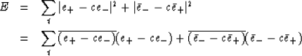
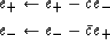
Now the error (13), which is the sum of the error of forward prediction plus the error of backward prediction, is minimized with respect to variation of c. (In a later chapter we will see fit to call c a reflection coefficient.) The quantity a remains fixed by the minimization of (11). Now let us establish that |c| is less than unity. Denote by e₊ the time series x_t + ax_t-1 which is the error in forward prediction of x_t. Denote by e_- the time series $x_{t-2} + \bar{a}x_{t-1}$ of error on backward prediction. With this, (13) becomes

$$\begin{eqnarray} E &= & \sum_t \vert e_+ - ce_-\vert^2 + \vert\bar{e}_- - c\bar{... ..._-) + \overline{(\bar{e}_- - c\bar{e}_+)}(\bar{e}_- - c\bar{e}_+)\end{eqnarray}$$ (14)

Setting the derivative with respect to $\bar{c}$ equal to zero

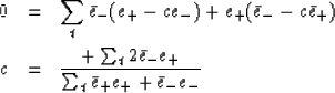$$\begin{eqnarray} 0 &= & \sum_t \bar{e}_- (e_+ - ce_-)+ e_+ (\bar{e}_- - c\bar{e}... ...sum_t 2\bar{e}_- e_+ \over \sum_t \bar{e}_+ e _+ + \bar{e}_- e_-}\end{eqnarray}$$ (15)

(One may note that $\partial E/\partial c = 0$ gives the same result.) That |c| is always less than unity may be seen by noting that the length of the vector $e_+ \pm e_-$ is always positive. In particular

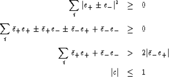$$\begin{eqnarray} \sum^{}_t \vert e_+ \pm e_-\vert^2 &\geq & 0 \nonumber \\ \su... ...gt & 2\vert\bar{e}_- e_+\vert \nonumber \\ \vert c\vert &\leq & 1\end{eqnarray}$$ (16)

If we now redefine e₊ and e_- as

$$\begin{eqnarray} e_+ \leftarrow e_+ - ce_- \\ e_- \leftarrow e_- - \bar{c}e_+\end{eqnarray}$$ (17) (18)

we have the forward and backward prediction errors of the three-term filter $(1, a'_1, a'_2) = (1, a_1 - c\bar{a}_1, -c)$.One can then return to (14) and proceed recursively. As the recursion proceeds e₊ and e_- gradually become unpredictable random numbers. We have then found a filter A(Z) which filters X(Z) either forward or backward and the output must be the inverse of the spectrum of the filter.

In later chapters we will discover a wave-propagation interpretation of the Burg algorithm. In a layered medium the parameters c_k have the interpretation of the up- and downgoing waves; and the whole process of calculating a succession of c_k amounts to downward continuing surface seismograms into the earth, determining an earth model c_k as you go.

EXERCISES:

1. Consider the time series with ten points (1, 1, 1, -1, -1, -1, 1, 1, 1, -1). Compute C and A up to cubics in Z. Compare the autocorrelation r_t calculated by Burg's method with R(Z) estimated from the truncated sample and with R(Z) estimated by intuitively extending the data sample in time to plus and minus infinity.
2. Modify the program of Figure  to compute and include the scale factor V which belongs in the spectrum.