GETTING THE REFLECTION COEFFICIENTS FROM THE WAVES

The best starting point for inverse problems is the Kunetz equation (19).  

$$1 + R \left( {1 \over Z} \right) + R(Z) \eq {Y_k \over Y_1} E \left( {1 \over Z} \right) E(Z)$$ (50)

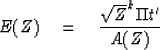
We need also the expression for the escaping wave (41)  

$$E(Z) \eq {\sqrt{Z}^k \Pi t' \over A(Z)}$$ (51)

We also need to recall that $Y_k /Y_1 = \Pi t/t'$. With this (50) becomes  

$$1 + R(Z) + R \left( {1 \over Z} \right) \eq {\Pi t't \over A(Z)A(1/Z)}$$ (52)

Multiplying through by A(Z) we get  

$$\left[ 1 + R(Z) + R \left( {1 \over Z} \right) \right] A(Z) \eq {\Pi t't \over A(1/Z)}$$ (53)

Since A(Z) is minimum-phase, A(Z) may be written as 1/B(Z) or A(1/Z) = 1/B(1/Z). Thus (53) becomes

$$[1 + R(Z) + R(1/Z)] A(Z) \eq (\Pi t't) \left( 1 + {b_1 \over Z} + {b_2 \over Z^2} + \cdots \right)$$ (54)

Identifying coefficients of zero and positive powers of Z as simultaneous equations, we get a set of equations which for a three-layer model looks like (r₀ = 1).  

$$\left[ \begin{array} {cccc} r_0 & r_1 & r_2 & r_3 \\ r_1 &... ...\\ 0 \\ 0 \\ 0 \\ 0 \\ \cdot \\ \cdot \end{array} \right]$$ (55)

In (55) we see our old friend the Toeplitz matrix. It used to work for factoring spectra and predicting time series. Notice that -c₃ has been inserted in (55) as the highest coefficient of A(Z). This is justified by reference back to the definition of A(Z) in terms of F(Z) and G(Z) which were in turn defined from the c_k. It is by reexamining the Toeplitz simultaneous equations (55) and the Levinson method of solution () that we will learn how to compute the reflection coefficients from the waves.

The first four equations in (55) would normally be thought of as follows: Given the first three reflected pulses r₁,r₂, and r₃ we may solve the equations for A, incidentally getting the reflection coefficient c₃. Knowing A, the 5th equation in (55) may be used to compute r₄. If the model were truly a three-layer model, it would come out right; if not, the discrepancy would be indicative of another reflector c₄ which could be found by expanding equation (55) from 4th order to 5th order. In summary, given the reflected pulses r_k, the Levinson recursion successively turns out the reflection coefficients c_k.

Now suppose we begin by observation of the escaping wave E(Z). One way to determine the reflection coefficients would be to form 1 + R(Z) + R(1/Z) by the autocorrelation of E(Z); then, the Levinson recursion could be used to solve for the reflection coefficients. The only disadvantage of this method is that E(Z) contains an infinite number of coefficients so that in practice some truncation must be done. The truncation is avoided by an alternative method. Given E(Z) polynomial division will find A(Z). The heart of the Levinson recursion is the building up of A(Z) by A_k(Z) = A_k-1(Z) - c_k Z^kA_k-1(1/Z). In particular, from () we have  

$$\left[ \begin{array} {l} 1 \\ a_1 \\ a_2 \\ a_3 \end{arr... ...begin{array} {l} 0 \\ a_2 \\ a_1 \\ 1 \end{array} \right]_2$$ (56)

which shows how to get A₃(Z) from A₂(Z) and c₃. To do it backwards, we see first that c₃ is -a₃. Then write (56) upside-down  

$$\left[ \begin{array} {l} a_3 \\ a_2 \\ a_1 \\ 1 \end{arr... ...begin{array} {l} 1 \\ a_1 \\ a_2 \\ 0 \end{array} \right]_2$$ (57)

Next multiply (56) by 1/(1 - c₃²) and add the product to (57) multiplied by c₃/(1 - c₃²). Notice that the upside-down vectors on the right-hand side cancel, leaving  

$${1 \over 1 - {c_3}^2} \left[ \begin{array} {l} 1 \\ a_1 \\... ...begin{array} {l} 1 \\ a_1 \\ a_2 \\ 0 \end{array} \right]_2$$ (58)

Equation (58) is the desired result which shows how to reduce A_k+1(Z) to A_k(Z) while learning c_k+1. A program to continue this process is

       COMPLEX A,C,AL,BE,TOP,CONJG
       C(1)=-1.; R(1)=1.; A(1)=1.; V(1)=1.
 300   DO 310 I=1,N
 310   C(I)=A(I)
       DO 330 K=1,N
       J=N-K+2
       AL=1./(1.-C(J)*CONJG(C(J)))
       BE=C(J)*AL
       JH=(J+1)/2
       DO 320 I=1,JH
       TOP=AL*C(I)-BE*CONJG(C(J-I+1))
       C(J-I+1)=AL*C(J-I+1)-BE*CONJG(C(I)) 
 320   C(I)=TOP
 330   C(J)=-BE/AL

A program to compute reflection coefficients c_k from the prediction-error filter A(Z). The complex arithmetic is optional.

An inverse program to get R and A from c is

       COMPLEX C,R,A,BOT,CONJG
       C(1)=-1.; R(1)=1.; A(1)=1.; V(1)=1.
 100   DO 120 J=2,N
       A(J)=0.
       R(J)=C(J)*V(J-1)
       DO 110 I=2,J
 110   R(J)=R(J)-A(I)*R(J-I+1)
       JH=(J+1)/2
       DO 120 I=1,JH
       BOT=A(J-I+1)-C(J)*CONJG(A(I))
       A(I)=A(I)-C(J)*CONJG(A(J-I+1))
 120   A(J-I+1)=BOT

This program computes both R and A from c.

 

8-12 Figure 12 Earthquake seismogram geometry with white light incident from below. In the top layer, the sum of the waves vanishes representing zero pressure at the free surface. The difference of up- and down- is the observed vertical component of velocity.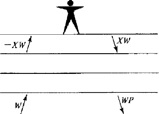

Finally, let us see how to do a problem where there are random sources. Figure 12 shows the ``earthquake geometry." However, in order to introduce a statistical element, the pulse incident from below has been convolved with a white light series w_t of random numbers. Consequently, all the waves internal to Figure 12 are given by the convolution of w_t with the corresponding wave in the impulse incident model. Now suppose we are given the top-layer waves D = 1 -U = XW and wish to consider downward continuation. We have the layer matrix  

$$\left[ \begin{array} {c} U \\ D \end{array} \right]_{k+1} ... ...ght] \; \left[ \begin{array} {c} U \\ D \end{array} \right]_k$$ (59)

which can be re-written as  

$$\left[ \begin{array} {r} -U \\ D \end{array} \right]_{k+1}... ...ht] \; \left[ \begin{array} {c} -U \\ D \end{array} \right]_k$$ (60)

The Burg prediction-error scheme can be written in the form  

$$\left[ \begin{array} {l} e^+ \\ e^- \end{array} \right]_{k... ... \; \left[ \begin{array} {l} e^+ \\ e^- \end{array} \right]_k$$ (61)

which makes it equivalent within a scale factor to downward continuing surface waveforms. The remaining question is whether Burg's estimate of the reflection coefficient, namely,  

$$\hat c_k \eq {2 \sum_t e^+_k e^-_k \over \sum_t e^+_k e^+_k + e^-_k e^-_k}$$ (62)

turns out to estimate the reflection coefficient c_k in the physical model. To see how Burg's $\hat c_k$ is related to the c_k arising in the Levinson recursion, we define ${\bf f}^+$ and ${\bf f}^-$ for k=2 as  

$$\left[ \begin{array} {c} \\ \\ {\bf f}^+ \\ \\ \\ \end... ...; \left[ \begin{array} {l} 0 \\ a_1 \\ 1 \end{array} \right]$$ (63)

Next from the dot product

$$\begin{eqnarray} ({\bf f}^-)^T{\bf f}^+ &= & [0 \quad a_1 \quad 1] \left[ \begin... ...] \; \left[ \begin{array} {l} 1 \\ a_1 \\ 0 \end{array} \right]\end{eqnarray}$$ (64)

Now utilize the fact that (1,a₁) satisfies the $2 \times 2$ system. Following the Levinson recursion (64) can be written as  

$$({\bf f}^-)^T {\bf f}^+ \eq [0 \quad a_1 \quad 1] \left[ \begin{array} {c} v \\ 0 \\ e \end{array} \right] \; \eq e$$ (65)

Likewise we can deduce that ${\bf f}^+ \cdot {\bf f}^+ = {\bf f}^- \cdot {\bf f}^- = v$.Thus, the Levinson calculation of the reflection coefficient can be written as  

$$c \eq { 2({\bf f}^+ \cdot {\bf f}^-) \over ({\bf f}^+ \cdot {\bf f}^+) + ({\bf f}^- \cdot {\bf f}^-)} \eq {2e \over 2v}$$ (66)

The Burg treatment differs from the Levinson treatment in that Burg omits end-effect terms on (63). Instead of (63) he has  

$$\left[ \begin{array} {c} e^+ \end{array} \\ \right] \; = \... ...ght] \; \left[ \begin{array} {l} a_1 \\ 1 \end{array} \right]$$ (67)

For a sufficiently long data sequence the Burg method and the Levinson technique thus become indistinguishable. For a data sample of finite duration we must make a choice. The Levinson technique with (63) is equivalent to assuming the data sample vanishes off the ends of the interval in which it is observed. In most applications this is untrue, and so the Burg technique is usually preferable.

EXERCISES:

1. An impulse and the first part of a reflection seismogram, that is, 1 + 2R(Z) is $1 + 2(Z/4 + Z^2/16 + Z^3/4 + \cdots)$.What are the first three reflection coefficients? Assuming there are no more reflectors what is the next point in the reflection seismogram?
2. A seismogram X(Z) = 1/(1 - .1Z + .9Z²) is observed at the surface of some layers over a halfspace. Sketch the time function and indicate its resonance frequency and decay time. Find the reflection coefficients if X(Z) is due to an impulsive source of unknown magnitude in the halfspace below the layers.
3. A source b₀ + b₁Z deep in the halfspace produces a seismogram $B(Z)X(Z) = 1 - Z + Z^2/2 - Z^3/2 + Z^4/4 - Z^5/4 + Z^6/8 - Z^7/8 + \cdots$.What are the layered structure and the source time function?