Model 2

The second model we use to illustrate our procedure is derived from the same synthetic structure. This model differs from the first in that we now assume that we have no information about both the lower and the upper parts of the layer. The aim of this model is to recover the slowness anomaly, both in the upper and the lower sections.

For this second model, we follow the same basic steps as for the previous model. Here are the results:

1.

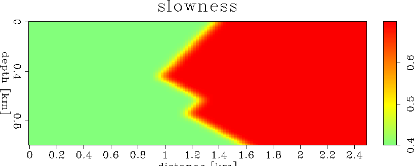
Figure 21 represents the background slowness model. The fast layer is missing completely in this example.

 

mod2.Slow.1 Figure 21 The starting slowness for model 2. It represents the background during the first pass (Figure 2).

2.

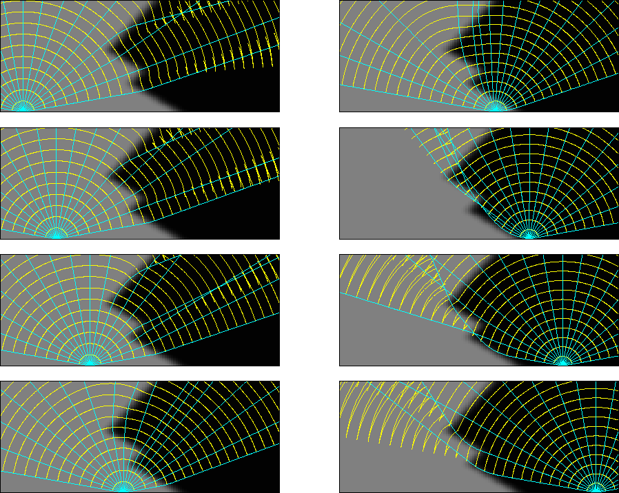
Figure 22 represents rays and wavefronts for different shooting locations in the subsurface. The background wavefield is distorted, but not as much as in the case of the first model. This would indicate that this example is easier than the first one, although it probably doesn't make a significant difference because WEMVA handles naturally complex wavefields.

 

mod2.rays Figure 22 Rays and wavefronts for different source points in the subsurface. The wavefield for model 2 also triplicates because of the slowness variation in the background, but not as strongly as in the case of the first model.

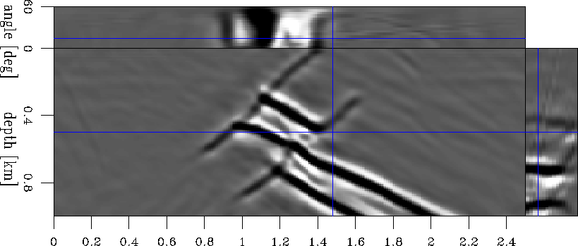
3.

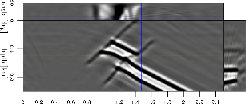
Figure 23 is the background image for model 2. Correctly migrated events are flat, while the incorrect ones are not. The background image is similar to the one in the preceding example (Figure 8), but it is distorted more, especially in the upper segment of the faulted layer.

 

mod2.bimg.1 Figure 23 The background image for model 2 presented as angle-domain common image gathers. Correctly migrated events are flat, while the incorrect ones are not.

4.

Figure 24 is the image enhanced by residual migration. Figure 25 is the corresponding picked velocity ratio surface.

 

mod2.aimg.1 Figure 24 The enhanced image for model 2.

 

mod2.lmap.1 Figure 25 The picked velocity ratio surface for model 2.

5.

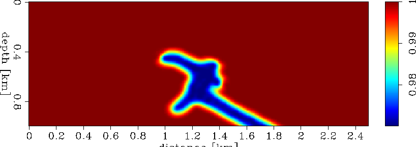
Figure 26 is the image perturbation computed from the background image (Figure 23) and the image enhanced by residual migration (Figure 24). For comparison, Figure 27 is the image perturbation obtained through the difference of the images migrated with the true and background slowness functions.

 

mod2.dimg.1 Figure 26 The image perturbation for model 2 computed from the background image and the image enhanced by residual migration.

 

mod2.dimg.0 Figure 27 The image perturbation for model 2 computed from the background image and the image obtained through migration with the true slowness.

6.

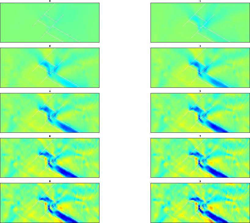
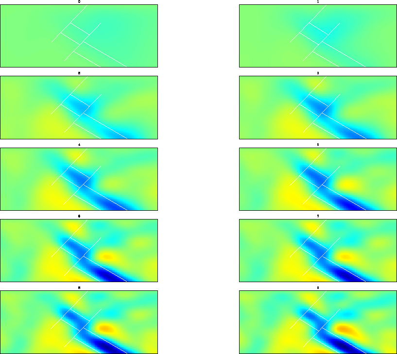
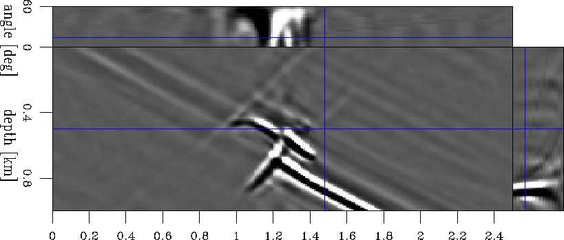
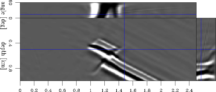
Figure 28 are the iteration panels for unregularized inversion, and Figure 29 are the iteration panels for preconditioned inversion. Here we can see the major differences and similarities between this and the first example: the lower part of the layer is well recovered; the upper part of the layer is also recovered reasonably well, although not as well as the lower part. The region around the fault, however, is not constrained enough and shows high spatial-frequency variation in slowness (Figure 28). However, if we regularize the model during the inversion, we recover a much smoother anomaly. The most significant change occurs in the area surrounding the fault. In this case, we do not observe the large fluctuations that occur in the unregularized example, although the regularization operator causes the slowness anomaly to leak outside its bounds.

 

mod2.inv.plain.1
Figure 28 Iteration panels for the unregularized inversion in the case of model 2.

 

mod2.inv.laplacian.1
Figure 29 Iteration panels for the preconditioned inversion in the case of model 2.

7.

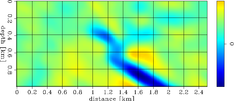
Figure 30 is the unregularized solution after the first loop, and Figure 31 is the solution after the first loop when the model is regularized using steering filters. The second of the two is a significantly improved result: the anomaly is much smoother, and the leakage in the vertical direction outside the layer bounds is reduced compared to the case of preconditioning with an isotropic Laplacian operator.

 

mod2.sol.plain.1 Figure 30 Unregularized solution for model 2 after the first loop.

 

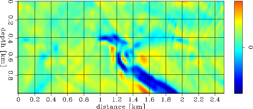mod2.sol.steering.1 Figure 31 Solution for model 2 after the first loop in the case of regularization with steering filters.

8.

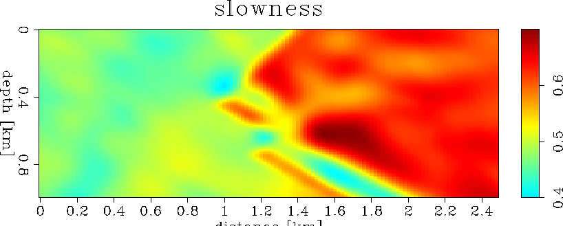
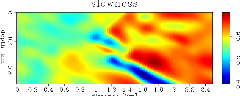
Figure 32 is the updated background slowness after the first loop, and Figure 33 is the corresponding updated background image. Although not yet completely there, the fast layer begins to build-up, and, consequently, the quality of the migrated image improves. However, we have not reached a satisfactory image at every location; therefore, we need to repeat the WEMVA loop. When we repeat the loop we obtain the slowness perturbation shown in Figure 34 and the updateded image shown in Figure 35.

 

mod2.Slow.2 Figure 32 Updated background slowness for model 2 after the first loop. The line search procedure gives the slowness perturbation scaling parameter $\alpha=1.64043$.

 

mod2.bimg.2 Figure 33 The updated background image for model 2 after the first loop.

 

mod2.Slow.3 Figure 34 Updated background slowness for model 2 after the second loop. The line search procedure gives the slowness perturbation scaling parameter $\alpha=2.81967$.

 

mod2.bimg.3 Figure 35 The updated background image for model 2 after the second loop.

The main conclusions we can derive from the second example are:

• Residual migration is successful in producing a good image perturbation, even though the starting image is more complex and significantly more distorted than in the first case.
• The anomaly produced by WEMVA without model regularization does not have as high a quality as it does in the original case. Large distortions in the original image, possibly coupled with residual migration distortions, lead to high spatial frequency variations of the inverted anomaly. We can, however, control the shape of the anomaly with smoothness constraints on the model, among which steering filters produce a promising result.
• The updated image is characterized by flatter angle-domain common image gathers. One loop, however, doesn't seem to be enough to achieve a completely satisfactory result, and we need to iterate more.