Model 1

As specified earlier, for model 1 we assume we do not have any information about the lower part of the fast velocity layer, but that we know the geometry and magnitude of the slowness in the upper segment. Figure 6 depicts the starting (background) slowness model. The background wavefield is significantly distorted by the strong slowness variation in the background, as shown in Figure 7.

 

mod1.Slow.1 Figure 6 The starting slowness for model 1. This slowness model represents the background during the first pass (Figure 2).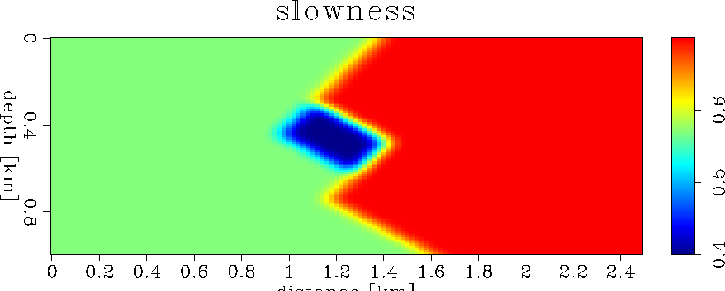

 

mod1.rays Figure 7 Rays and wavefronts for different source points in the subsurface. The wavefield triplicates because of the strong slowness variation in the background.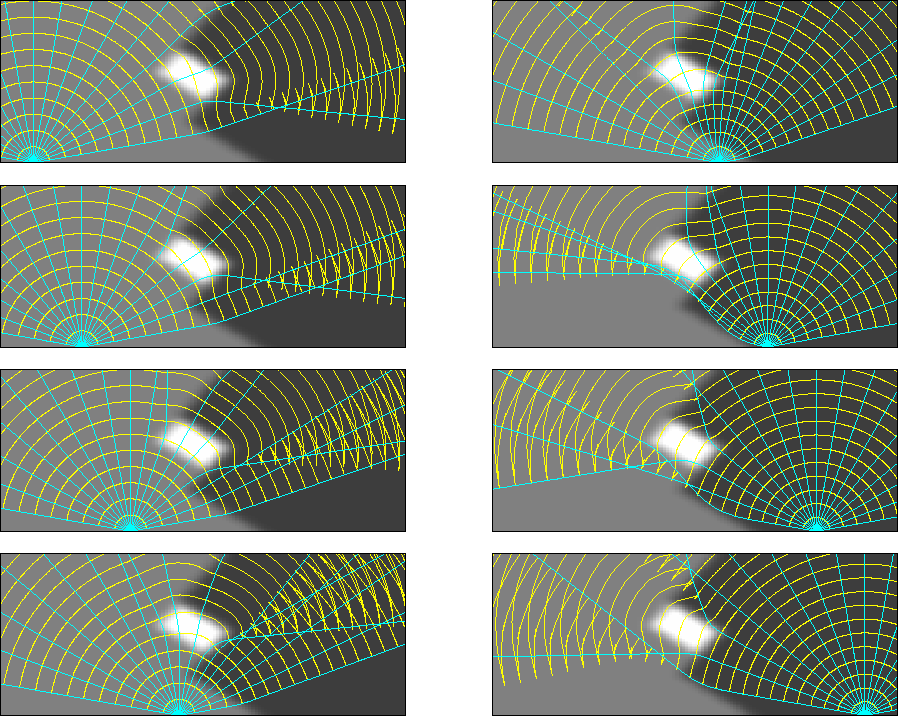

Next, we migrate the synthetic data using the background slowness. The resulting image (Figure 8) is perfect in the upper part of the section, above the area with inaccurate slowness, but it is not completely accurate in the lower part, where the incorrect slowness model limits our imaging abilities. To analyze the quality of the image, we display it as angle-domain common image gathers Prucha et al. (1999); Sava and Fomel (2000) that have the property of showing flat events when the migration velocity is correct, and bending events when the velocity is incorrect.

 

mod1.bimg.1 Figure 8 The background image for model 1 presented as angle-domain common image gathers. The correctly migrated events are flat, while those incorrectly migrated are not, for example at the bottom of the lower layer.

In the next step, we compute an improved image (Figure 9) following the methodology outlined earlier in this paper and fully described in Sava (1999). As expected, there is no improvement in the upper section, since the velocity model is correct there, but only in the lower section, under the fault region. The picked velocity ratio surface is presented in Figure 10.

 

mod1.aimg.1 Figure 9 The enhanced image for model 1.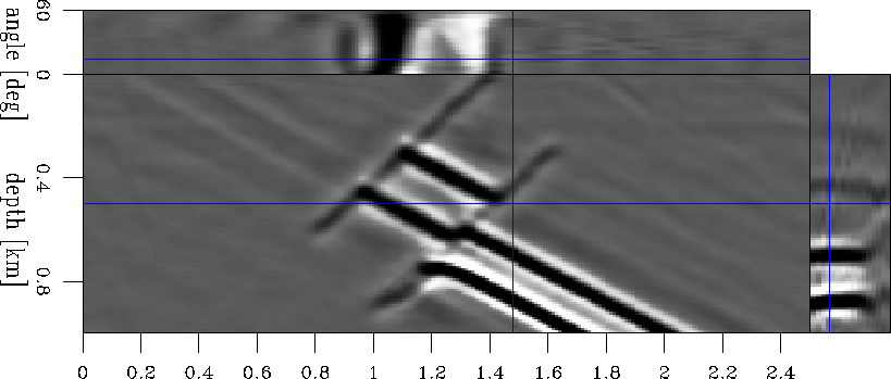

 

mod1.lmap.1 Figure 10 The picked velocity ratio surface for model 1. This surface has values different from 1 only in the areas where the image has changed as a result of residual migration.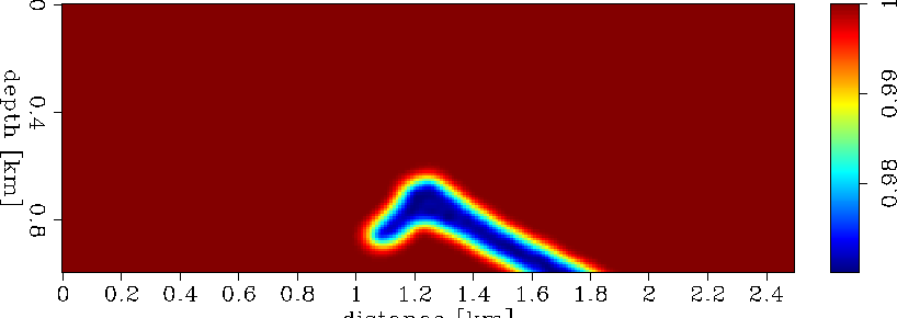

Finally, we can take the background (Figure 8) and enhanced (Figure 9) images and compute the image perturbation, depicted in Figure 11. For comparison, Figure 12 shows the theoretically-correct image perturbation computed using the true slowness to migrate the data. Although the two images are not identical, they are similar. In practice, our goal is to come as close as possible to the image in Figure 12.

 

mod1.dimg.1 Figure 11 The image perturbation for model 1 computed from the background image and the image enhanced by residual migration.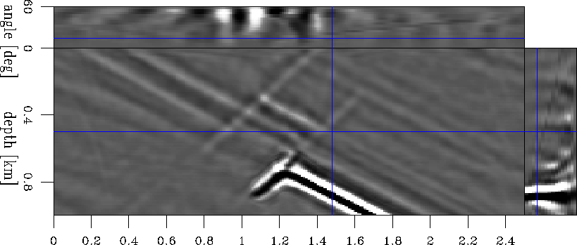

 

mod1.dimg.0 Figure 12 The perturbation in image for model 1 computed from the background image and the image obtained through migration with the true slowness.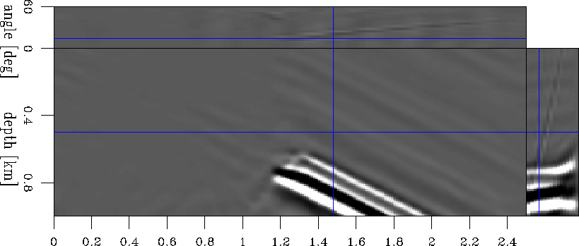

We have reached the point where we have created an image perturbation. We can now go one step further and compute the perturbation in slowness by solving the least-squares systems in Equations (1) or (2).

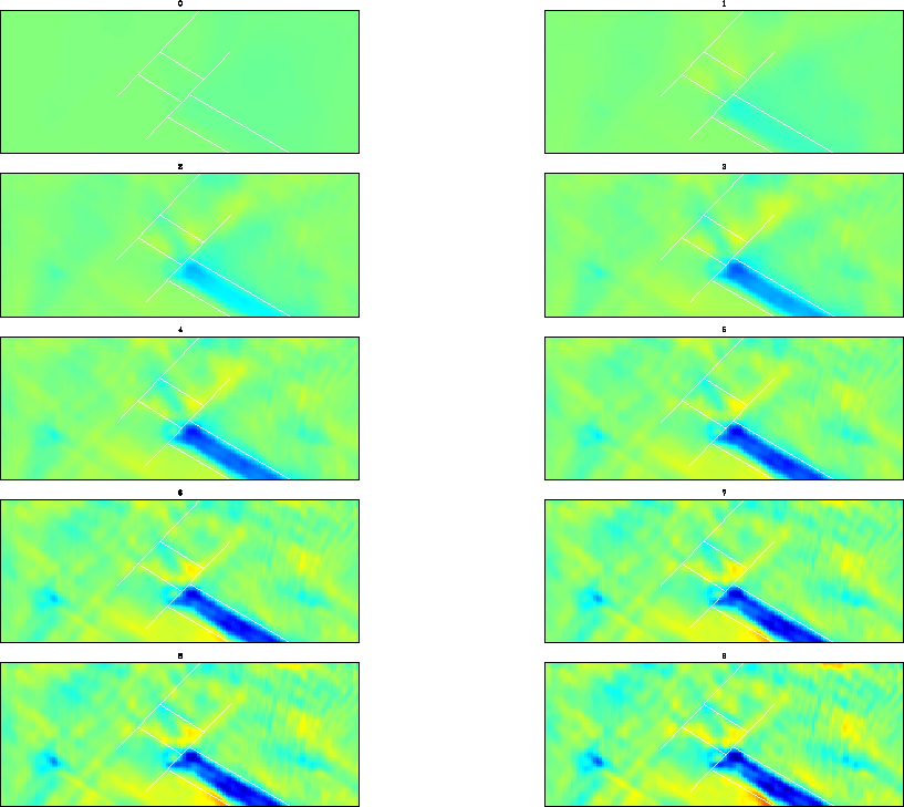
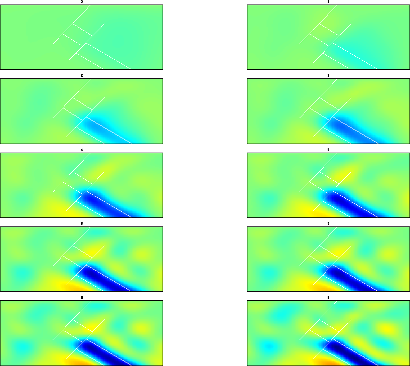
Figure 13 shows the result of the inversion process without any model regularization [$\epsilon=0$ in equation (2)]. Every panel in the figure represents one iteration, as indicated by its title. The anomaly we seek is nicely recovered, with its position confined to the right area, as indicated by the schematic overlay. The absolute magnitude of the anomaly is smaller than that of the true one. This result can probably be explained by the nature of the Born approximation and the scaling of the velocity ratio surface. The definitive answer, however, is subject to further research.

Even though we have not yet imposed any smoothness constraint on the model, the anomaly is reasonably smooth, which is a direct consequence of the band-limited character of our wave-equation processing. The image is also free of major artifacts, although the bottom area of the model, which is not constrained by anything in the image perturbation, develops an anomaly of the opposite sign and another small, blob-like anomaly, possibly a wrap-around artifact.

 

mod1.inv.plain.1
Figure 13 Iteration panels for the unregularized inversion in the case of model 1.

 

mod1.sol.plain.1 Figure 14 Unregularized solution for model 1 after the first loop.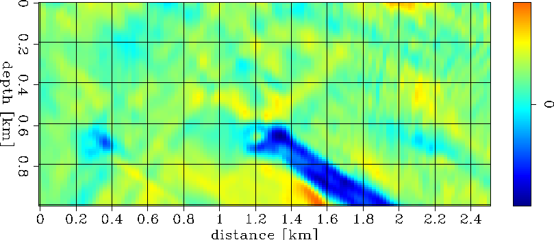

Figure 15 shows the result of model inversion for the regularized system (Equations 1). The anomaly is even smoother and confined to its correct location. Figures 14 and 16 show the final inversion result for the unregularized case and the case of preconditioning the model with a steering filter that forces the data to spread more along the geological dip and less perpendicular to it.

 

mod1.inv.laplacian.1
Figure 15 Iteration panels for the preconditioned inversion in the case of model 1.

 

mod1.sol.steering.1 Figure 16 Solution for model 1 after the first loop in the case of regularization with steering filters.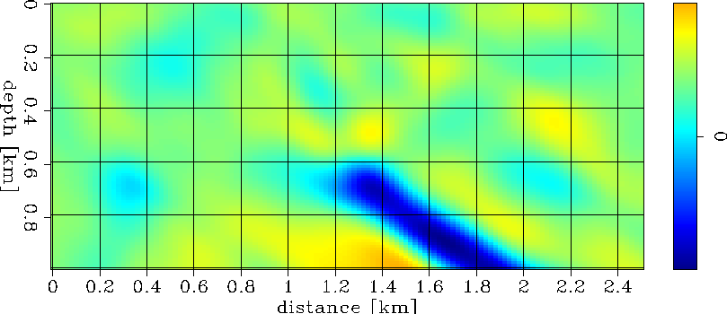

Finally, we update the background slowness model and repeat the loop. Figure 17 shows the updated background slowness, and Figure 18 the new background image. This new image should be compared to the previous background image (Figure 8). Notably, the bottom layer is pushed in depth closer to its correct position, and the angle-domain common image gathers show, on the average, flatter events, indicating that the new image is migrated with better velocity. The slowness perturbation is scaled differently before summation, as guided by the line-search optimization (Equation 3). We repeat the loop and obtain the slowness perturbation shown in Figure 19 and the updateded image shown in Figure 20.

 

mod1.Slow.2 Figure 17 Updated background slowness for model 1 after the first loop.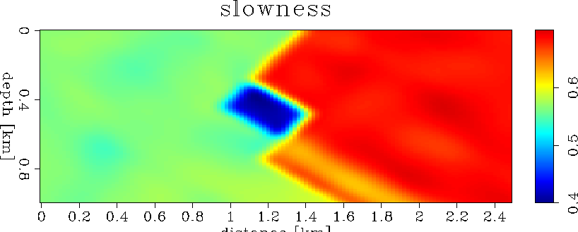

 

mod1.bimg.2 Figure 18 The updated background image for model 1 after the first loop.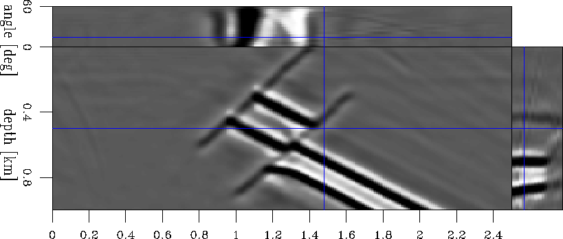

 

mod1.Slow.3 Figure 19 Updated background slowness for model 1 after the second loop. The line search procedure gives the slowness perturbation scaling parameter 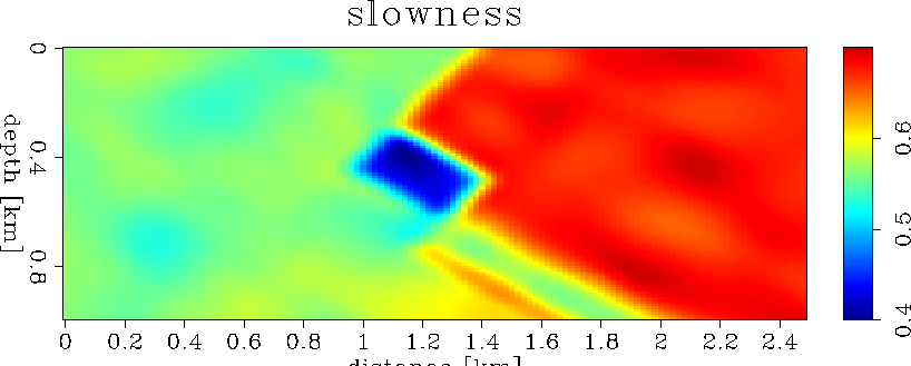$\alpha=0.625977$.

 

mod1.bimg.3 Figure 20 The updated background image for model 1 after the second loop. The line search procedure gives the slowness perturbation scaling parameter 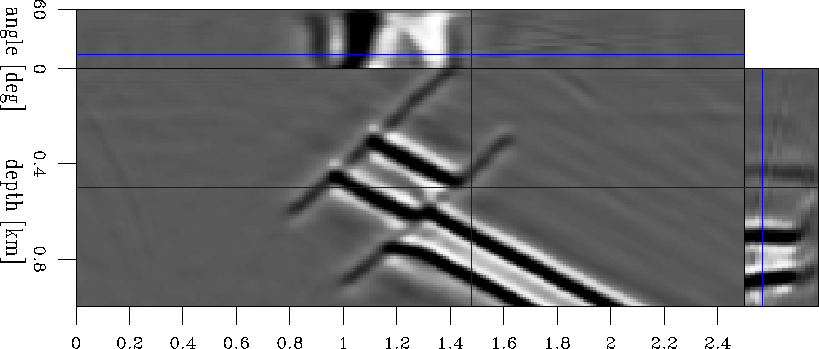$\alpha=1.0262$.

Here are the main conclusions we can derive from the first example:

• The image perturbation produced with residual migration is reasonably good, even for the case of a model with significant wavefield distortions in the background.
• As expected, wave-equation inversion produces smooth results, because of the intrinsic band-limited nature of wave propagation. Model regularization, however, helps to produce an even smoother slowness perturbation.
• The magnitude of the slowness anomaly we produced after inversion is less than the correct one. This is, in part, explained by the various approximations made when we created the image perturbation. It remains, nevertheless, an interesting topic that requires further investigation.
• The updated background slowness is able to produce an improved image, measured by the flatness of the angle-domain common image gathers. In other words, we have fulfilled the main goal of our procedure - image improvement- at the same time that we have improved the slowness model.
• Two WEMVA loops do not seem to be enough to recover the full slowness perturbation. We can get better results if we loop more, although cost remains a significant limitation. Here we have another direction of future work.