


Next: 3-D ALGORITHM
Up: THE BASIC FINITE-DIFFERENCE SCHEME
Previous: THE BASIC FINITE-DIFFERENCE SCHEME
The practical implementation of the above formulation is centered
around the problem of advancing the computational front.
The Engquist-Osher scheme provides a way to compute  by
imposing a time minimization condition along three points of the
finite-difference stencil.
The scheme calculates
by
imposing a time minimization condition along three points of the
finite-difference stencil.
The scheme calculates
 to approximate the partial derivative
(with respect to
to approximate the partial derivative
(with respect to  ), of the
function
), of the
function  , by using the values of in points of minimum traveltime; varies only in
along the constant radius computational front.
Given three consecutive points on the computational front with
constant radius, the values of the functions
, by using the values of in points of minimum traveltime; varies only in
along the constant radius computational front.
Given three consecutive points on the computational front with
constant radius, the values of the functions
 and vary only in the variable .Each function will have the values uj-1, uj, uj+1
and vj-1, vj and vj+1 respectively, in the three points
of the stencil.
From equation (6) we can write as
a function of :
and vary only in the variable .Each function will have the values uj-1, uj, uj+1
and vj-1, vj and vj+1 respectively, in the three points
of the stencil.
From equation (6) we can write as
a function of :
The Engquist-Osher scheme computes as
|  |
(7) |
where  , at the point where
 . For this case
the value of
. For this case
the value of 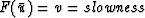 from equation (6).
Because the values of uj-1, uj and uj+1 are
compared against zero (), the scheme needs only the
sign of the function u in the three points of the stencil.
Equation (7) allows for eight cases as a function of the
positive or negative values of uj-1, uj and uj+1 in
the three points of the stencil.
The eight cases are shown in Figure 1.
from equation (6).
Because the values of uj-1, uj and uj+1 are
compared against zero (), the scheme needs only the
sign of the function u in the three points of the stencil.
Equation (7) allows for eight cases as a function of the
positive or negative values of uj-1, uj and uj+1 in
the three points of the stencil.
The eight cases are shown in Figure 1.
Figure 1:
Eight possible cases for the Engquist-Osher scheme. The thick
vertical bars
represent the sign of  , the
continuous line represents the values of the traveltime over the
three points of the stencil, the dashed vertical lines represent
the location where
, the
continuous line represents the values of the traveltime over the
three points of the stencil, the dashed vertical lines represent
the location where
 ; the dots on the
time line show the coordinates for the function
which contribute to the difference .On the right side are the values for
the computed for each case.
; the dots on the
time line show the coordinates for the function
which contribute to the difference .On the right side are the values for
the computed for each case.
|
The calculation of is done for locations
where the value of the traveltime function  , is
minimum. From Figure 1 one can see that only cases 1 and 5 will actually
give a first order correct value. In both cases the values
for the function v are chosen from the three points of the
stencil where the value of the time is minimum.
While for cases 1 and 5 the accuracy of the scheme is
unquestionable, for the rest of the cases some
approximations are introduced.
The other six cases also calculate the values of
using the points where the value of the time is minimum.
However,
the value of is divided by a constant
, is
minimum. From Figure 1 one can see that only cases 1 and 5 will actually
give a first order correct value. In both cases the values
for the function v are chosen from the three points of the
stencil where the value of the time is minimum.
While for cases 1 and 5 the accuracy of the scheme is
unquestionable, for the rest of the cases some
approximations are introduced.
The other six cases also calculate the values of
using the points where the value of the time is minimum.
However,
the value of is divided by a constant  ,even though the function is estimated over
a different interval .A potentially more accurate algorithm would calculate
the exact value of for each intermediate
case.
The algorithm can be
designed to calculate the locations of the minimum
travel time in the three point stencil interval and the
span over the axis, necessary to divide the value
.
,even though the function is estimated over
a different interval .A potentially more accurate algorithm would calculate
the exact value of for each intermediate
case.
The algorithm can be
designed to calculate the locations of the minimum
travel time in the three point stencil interval and the
span over the axis, necessary to divide the value
.
Next: 3-D ALGORITHM
Up: THE BASIC FINITE-DIFFERENCE SCHEME
Previous: THE BASIC FINITE-DIFFERENCE SCHEME
Stanford Exploration Project
12/18/1997