


Once I have estimated ![]() ,
an inverse problem for three isotropic elastic
parameters can be posed. Under the assumption that relative contrasts
in material properties are small at reflecting boundaries, and the reflection
angles are well within the pre-critical region (Aki and Richards, 1980),
a linearization of the
Zoeppritz plane wave reflection coefficients can be made at every subsurface
point
,
an inverse problem for three isotropic elastic
parameters can be posed. Under the assumption that relative contrasts
in material properties are small at reflecting boundaries, and the reflection
angles are well within the pre-critical region (Aki and Richards, 1980),
a linearization of the
Zoeppritz plane wave reflection coefficients can be made at every subsurface
point ![]() :
:
| |
(15) |
where ![]() are the relative contrasts in P impedance,
S impedance and
density at the reflecting boundary, and
are the relative contrasts in P impedance,
S impedance and
density at the reflecting boundary, and ![]() are known basis
functions which are analytical in
are known basis
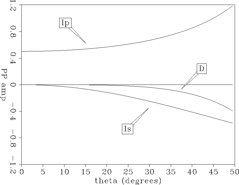
functions which are analytical in ![]() . The three basis functions
are plotted in Figure
. The three basis functions
are plotted in Figure ![[*]](http://sepwww.stanford.edu/latex2html/cross_ref_motif.gif) , with c1 at the top,
c2 at the bottom,
and c3 near the zero axis in the middle, and are given here analytically as:
, with c1 at the top,
c2 at the bottom,
and c3 near the zero axis in the middle, and are given here analytically as:
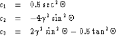 |
||
| (16) |
where ![]() is the shear to compressional velocity ratio vs/vp.
I used a constant value of
is the shear to compressional velocity ratio vs/vp.
I used a constant value of ![]() in this data example, but
it could be specified as a function
in this data example, but
it could be specified as a function ![]() if the appropriate
vp and vs information is available. In fact, the basis functions
ci are not too sensitive to reasonable ranges of
if the appropriate
vp and vs information is available. In fact, the basis functions
ci are not too sensitive to reasonable ranges of ![]() values.
values.
In principle, any three elastic parameters ![]() can be chosen that
span the
can be chosen that
span the ![]() space. I choose the elastic impedance parameterization,
because of its robust inversion properties for surface seismic geometries
when a narrow (e.g., 5-35) reflection illumination aperture is only
available in the data. I explored this issue more completely in
Lumley and Beydoun (1991), and it has recently become an active area of
discussion in AVO inversion (e.g., De Nicolao et al., 1991).
space. I choose the elastic impedance parameterization,
because of its robust inversion properties for surface seismic geometries
when a narrow (e.g., 5-35) reflection illumination aperture is only
available in the data. I explored this issue more completely in
Lumley and Beydoun (1991), and it has recently become an active area of
discussion in AVO inversion (e.g., De Nicolao et al., 1991).
In particular, I invert (15) at every subsurface location ![]() by a least-squares method which bootstraps with offset and angle.
The logic behind my approach is based on the properties of the basis functions
by a least-squares method which bootstraps with offset and angle.
The logic behind my approach is based on the properties of the basis functions
![]() , as plotted in Figure .
I first find a least-squares estimate for Ip using only
, as plotted in Figure .
I first find a least-squares estimate for Ip using only ![]() values
for which
values
for which ![]() . Next, I find a least-squares estimate for
Is using the
. Next, I find a least-squares estimate for
Is using the ![]() data in the range
data in the range ![]() and using the estimate of Ip as a constraint on the system.
Finally, if there are angles in the data greater than 35, I perform
a least-squares estimate for the density parameter using the Ip and
Is values as constraints. I have found this method to be a very robust
procedure for estimating Ip and Is (e.g., better than damped SVD),
and also for demonstrating that little or
no independent information on the contribution of density
contrasts to a reflection in typical surface seismic geometries is
invertible.
and using the estimate of Ip as a constraint on the system.
Finally, if there are angles in the data greater than 35, I perform
a least-squares estimate for the density parameter using the Ip and
Is values as constraints. I have found this method to be a very robust
procedure for estimating Ip and Is (e.g., better than damped SVD),
and also for demonstrating that little or
no independent information on the contribution of density
contrasts to a reflection in typical surface seismic geometries is
invertible.
 |


