


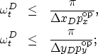
Figure 9 and
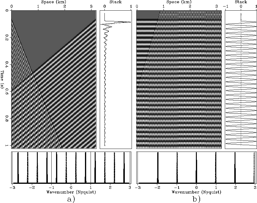
Figure 10
show two plane waves.
The plane waves are
adequately sampled when the waveform is
a 30 Hz sinusoid (Figure 9a),
but the one with positive time dip is aliased when the waveform is
a 60 Hz sinusoid (Figure 10a).
The data aliasing can be observed both in the
time-space domain, where the data appears to be dipping
in the opposite direction, and in the wavenumber domain.
The corresponding spatial spectra are shown
at the bottom of the Figures.
The solid lines correspond to the positive-dip
plane wave,
and the dotted line to the negative-dip plane wave.
The spectrum for the positive-dip plane wave (solid line)
at the bottom of Figure 9a
shows two spikes at ![]() replicated
at
replicated
at ![]() .Because of the doubling of the temporal frequency,
in the spectrum at the bottom of Figure 10a
the aliased spikes at
.Because of the doubling of the temporal frequency,
in the spectrum at the bottom of Figure 10a
the aliased spikes at ![]() moved into the central band to
moved into the central band to ![]() .
.
Data summation along a given trajectory is equivalent to a two-step process; first the data are shifted to align the events along the desired trajectory. Second, the traces are stacked together. In the case of the slant-stack operator, the summation trajectories are lines and the first step is equivalent to the application of linear moveout (LMO) with the desired dip. Figure 9b and Figure 10b show the results of applying LMO with the slowness of the positive-dip plane wave to the corresponding data in Figure 9a and Figure 10a. The traces on the right side of the sections are the results of stacking the corresponding data. At 30 Hz no aliasing occurs, and after LMO only the original plane wave stacks coherently, as desired. In contrast, at 60 Hz both plane waves stack coherently after LMO as well as the original plane wave. In general, artifacts are generated when data that are not aligned with the summation path stack coherently into the image. This phenomenon is the cause of the aliasing noise that degrades the image when operator aliasing occurs. To avoid adding aliasing noise to the image we could lowpass filter the input data according to the operator dips. The resulting anti-aliasing constraints are:
 |
||
| (3) |
 |


 |
 |
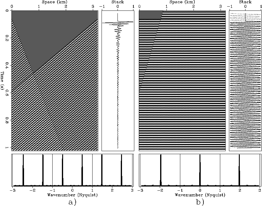
To further examine the idea of operator aliasing depending on the dip bandwidth in the data, we consider the two plane waves shown in Figure 11. In this case the two plane waves have a 60 Hz waveform, as in Figure 10, but with the second plane wave flat instead of dipping with a negative time dip. The two plane waves have conflicting dips; but the additional plane wave does not interfere with the stacking of the original plane wave even with a 60 Hz waveform.
The last two examples demonstrate that the limits on the dip range
for unaliased summation paths
are a direct function of the
expected dips in the data along the summation axes.
If ![]() and
and
![]() are respectively
the minimum and maximum dips expected in the data,
then, to avoid operator aliasing,
the operator dip must fulfill
the following inequalities:
are respectively
the minimum and maximum dips expected in the data,
then, to avoid operator aliasing,
the operator dip must fulfill
the following inequalities:
 |
||
| (4) |
 |
||
| (5) |
The data-dips limits
![]() and
and ![]() can be both spatially and time varying
according to the expected local dips in the data.
Therefore, the anti-aliasing filtering applied to the data
as a consequence of the constraints in equation (5)
can be fairly complex,
and dependent on: local dips, time, and spatial coordinates.
If no a priory knowledge on the local dips is available,
and the summation is carried out along the midpoint axes,
twice the inverse of propagation velocity is a reasonable bound
on the absolute values of both
can be both spatially and time varying
according to the expected local dips in the data.
Therefore, the anti-aliasing filtering applied to the data
as a consequence of the constraints in equation (5)
can be fairly complex,
and dependent on: local dips, time, and spatial coordinates.
If no a priory knowledge on the local dips is available,
and the summation is carried out along the midpoint axes,
twice the inverse of propagation velocity is a reasonable bound
on the absolute values of both ![]() and
and ![]() .In contrast, in the case that the summation is performed along the
offset axes, as for CMP stacks,
.In contrast, in the case that the summation is performed along the
offset axes, as for CMP stacks,
![]() can be safely assumed to be positive,
and at worst equal to zero.
In practice the bounds on the data's expected dips
should take into account all types of events,
and not only the dips of the reflections that we aim to image.
For example, in CMP gathers recorded on land,
can be safely assumed to be positive,
and at worst equal to zero.
In practice the bounds on the data's expected dips
should take into account all types of events,
and not only the dips of the reflections that we aim to image.
For example, in CMP gathers recorded on land,
![]() should take into account low-velocity events
such as ground roll.
should take into account low-velocity events
such as ground roll.
The most substantial benefits of applying the more
general constraints expressed
in equation (5)
are achieved when asymmetric bounds on the dips in the data
enable imaging without aliasing high-frequency components
that are present in the data as aliased energy,
and consequently would be filtered out if the constraints in
equation (3) were applied.
An important case when asymmetric bounds
on the data dips are realistic is the imaging
of steep salt-dome flanks,
as in the Gulf of Mexico data set shown above.
In this case, we can assume that the negative
time dips in the data are small.
According to the equations in (4),
the increase in ![]() raises the limit on
the maximum positive operator dip.
In practice, the application of the generalized
constraints in equation (5),
when
raises the limit on
the maximum positive operator dip.
In practice, the application of the generalized
constraints in equation (5),
when ![]() cause the migration operator to be asymmetric,
with dip bandwidth dependent on reflector direction.
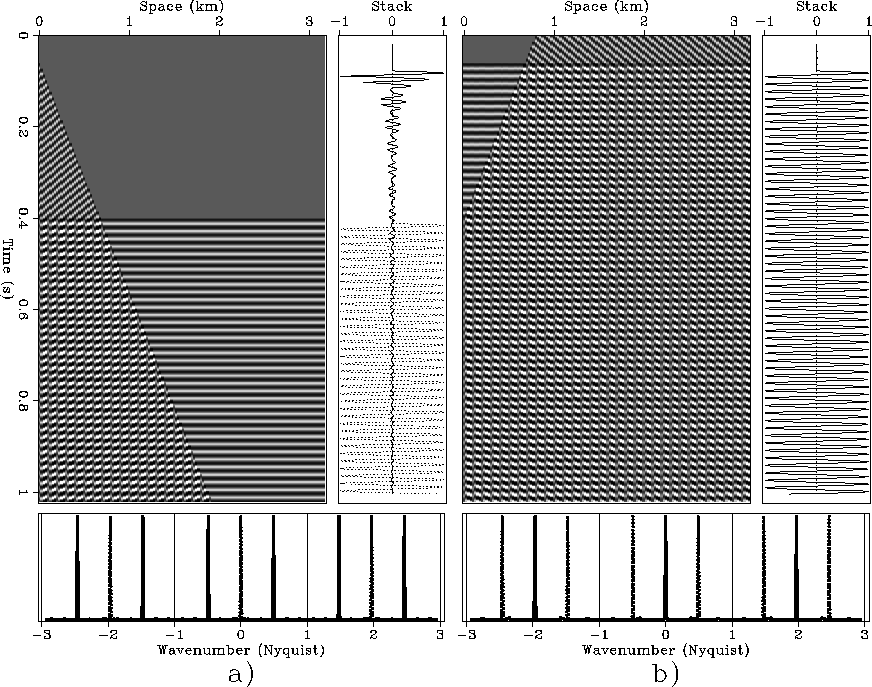
Figure 12
and
Figure 13
show an example of the effects of asymmetric
dip bounds on the migration operator.
For both images,
the image sampling is the same as
in Figure 6
cause the migration operator to be asymmetric,
with dip bandwidth dependent on reflector direction.
Figure 12
and
Figure 13
show an example of the effects of asymmetric
dip bounds on the migration operator.
For both images,
the image sampling is the same as
in Figure 6
![]() ,but the data sampling is assumed to
be coarser than the image sampling by a factor of two;
that is,
,but the data sampling is assumed to
be coarser than the image sampling by a factor of two;
that is,
![]() .When the constraints in equation (3)
are applied (see Figure 12),
the operator has lower resolution than in
Figure 6.
But if we assume that
.When the constraints in equation (3)
are applied (see Figure 12),
the operator has lower resolution than in
Figure 6.
But if we assume that ![]() ,and apply the constraints in equation (5)
(see Figure 13),
the positive time dips are imaged with the same resolution
as in Figure 6.
,and apply the constraints in equation (5)
(see Figure 13),
the positive time dips are imaged with the same resolution
as in Figure 6.
|
Imp-antialias-nodirect
Figure 12 Image obtained by applying Kirchhoff migration with ``standard'' anti-aliasing. Sampling rates are: | 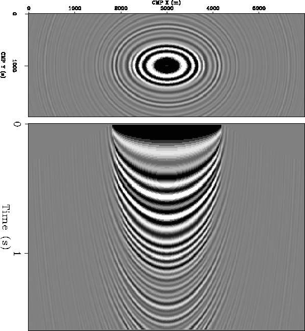 |
|
Imp-antialias-direct
Figure 13 Image obtained by applying Kirchhoff migration with ``directed'' anti-aliasing assuming | 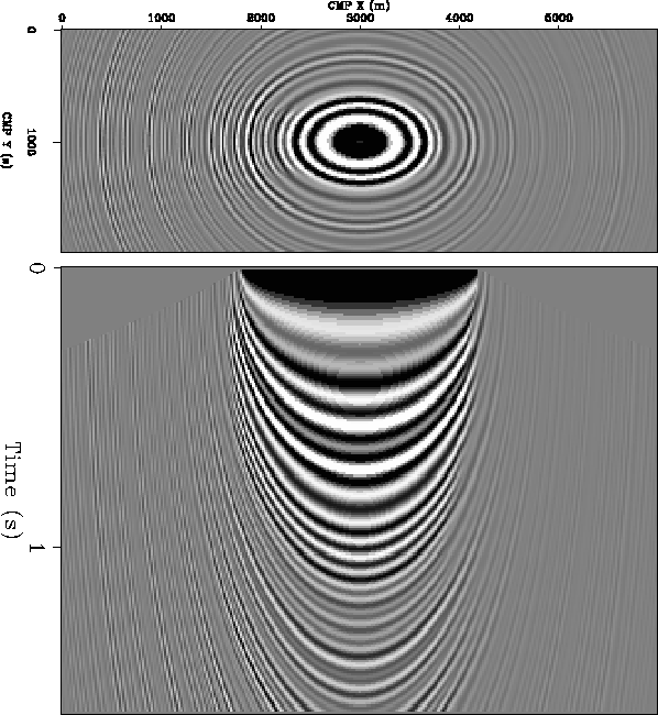 |