Analytical derivation

Another way to find the relation between z and z' starts from the cascade of two dispersion relations Biondi and Palacharla (1996). The first one is for 2-D prestack downward-continuation along the in-line direction,

$$k_z'= \sqrt{\frac{\omega^2}{v^2}-\frac{1}{4}(k_{m_x}+k_{h_x})^2}+ \sqrt{\frac{\omega^2}{v^2}-\frac{1}{4}(k_{m_x}-k_{h_x})^2},$$ (15)

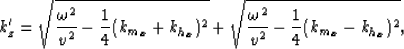
which is equivalent to equation (11). The second one is for 2-D zero-offset downward continuation along the cross-line axis,  

$$k_z = \sqrt{k_z'^2-k_{m_y}^2}$$ (16)

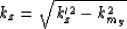
which is equivalent to equation (12). Indeed, by taking the square and dividing by k_z,

$$1=\frac{k_z'^2}{k_z^2} - \frac{k_{m_y}^2}{k_z^2}$$ (17)

and by introducing $\tan \delta = \frac{k_{m_y}}{k_z}$,

$$\frac{\partial z}{\partial z'}=\frac{k_z'}{k_z}= \sqrt{1+\tan^2 \delta}=\frac{1}{\cos \delta}.$$ (18)

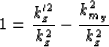
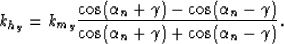
BThe coplanarity condition presented in Biondi and Palacharla (1996) is:

$$\hat k_{h_y}=k_{m_y}\frac {\sqrt{\frac{\omega^2}{v^2}-\frac{... ...+ \sqrt{\frac{\omega^2}{v^2}-\frac{1}{4}(k_{m_x}-k_{h_x})^2}}.$$ (19)

Each square root in the previous equation can be substituted with the expression including the dip angle of the source or the receiver ray

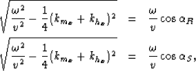$$\begin{eqnarray} \sqrt{\frac{\omega^2}{v^2}-\frac{1}{4}(k_{m_x}+k_{h_x})^2}&=& ... ...ac{1}{4}(k_{m_x}+k_{h_x})^2}&=& \frac{\omega }{v } \cos \alpha_S,\end{eqnarray}$$ (20) (21)

where $\alpha_S$ and $\alpha_R$ can be expressed in terms of the aperture angle $\gamma$ and the normal dip angle $\alpha_n$:

$$k_{h_y}=k_{m_y}\frac{\cos(\alpha_n+\gamma)-\cos(\alpha_n-\gamma)} {\cos(\alpha_n+\gamma)+\cos(\alpha_n-\gamma)}.$$ (22)

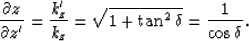
Or, after applying some trigonometric relations  

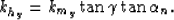$$k_{h_y}=k_{m_y}\tan \gamma \tan \alpha_n.$$ (23)

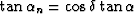We now introduce equation (2) as well as $\tan \alpha=\frac{k_{m_x}}{k_z}$ where $\alpha$ is the projection of the angle $\alpha_n$ on the vertical plane passing through the source-receiver axis. The two angles are linked by the relation $\tan \alpha_n = \cos \delta \tan \alpha$.Equation 23 becomes

$$k_{h_y}=\frac{k_{m_y}k_{m_x}k_{h_x}}{k_z^2+k_{m_y}^2}$$ (24)

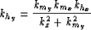
CConsider one image point in the Fourier domain, i.e. at given k_mx, k_my and k_z. For one image point, we have all the values of the offset gather. Each value is referenced in the Fourier domain by the offset wavenumbers k_hx and k_hy. Given a reflection azimuth $\beta$ and an aperture angle $\gamma$,we want to get the value of the sample associated with $\gamma$, hence what are the offset wavenumbers associated with $\gamma$.Given k_mx, k_my, k_z, $\beta$ and $\gamma$:

• Because of the reflection azimuth, we need to get into the new coordinates system. k'_mx, k'_my are computed using k_mx, k_my and $\beta$ in equation (4).
• For a given $\gamma$ and k_z we can determine k'_hx from equation (6).
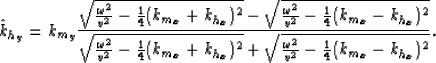
• The second component of the offset wavenumber, k'_hy, must satisfy the coplanarity condition (7).
• The two components of the offset wavenumber were obtained in the new system of coordinates. To return to the original system of coordinates, we use the inverse of transformations (4).
• We have determined which sample of the offset gather should be associated with the aperture angle $\gamma$.

The entire angle gather at the image point (k_mx, k_my, k_z) and at the reflection azimuth $\beta$ is obtained by looping over $\gamma$.