Next: Conclusion
Up: Attenuation of the ship
Previous: Abandoned strategy for attenuating
Now, I develop the new idea of removing the tracks by adaptively subtracting
them within our inversion scheme. Building on Chapter
![[*]](http://sepwww.stanford.edu/latex2html/cross_ref_motif.gif) , I introduce a modeling operator for the ship tracks
inside our fitting goal in equation () as follows:
, I introduce a modeling operator for the ship tracks
inside our fitting goal in equation () as follows:
| 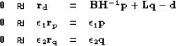 |
(42) |
where  is a drift modeling operator (leaky integration),
  is a
new variable of the inversion.
The following misfit function can then be minimized
is a
new variable of the inversion.
The following misfit function can then be minimized
|  |
(43) |
where  estimates the interpolated map of the lake.
Again, I set
estimates the interpolated map of the lake.
Again, I set  and do not iterate to
completion. The explicit elimination of the two regularization
parameters
and do not iterate to
completion. The explicit elimination of the two regularization
parameters  and
and  needs to be accounted
for. In practice, in the presence of crosstalks, they allow
us to put the common components of the data in whichever space we
choose. To accomodate my choice
of , a constant
needs to be accounted
for. In practice, in the presence of crosstalks, they allow
us to put the common components of the data in whichever space we
choose. To accomodate my choice
of , a constant  =
= is added to the modeling operator for the drift
(similar to equation () in Chapter ).
Then, for the operator , I choose a leaky integration operator
such that
is added to the modeling operator for the drift
(similar to equation () in Chapter ).
Then, for the operator , I choose a leaky integration operator
such that  is the portion
of data value
is the portion
of data value  that results from drift. Consistent with the
way I use a rough variable
that results from drift. Consistent with the
way I use a rough variable  to represent the smooth water
depth
to represent the smooth water
depth  , I now represent (for the purpose of speeding
iteration)
, I now represent (for the purpose of speeding
iteration)  by a rougher function
  .The operator
  has the following recursive form
|  |
(44) |
The parameter  controls the decay of the integration.
For
controls the decay of the integration.
For  , leaky integration represents causal integration.
The operator is then appropriate to model the secular
variations implied by the different season and human conditions
during the data acquisition. We simply have to choose a value of
that best represents the variations between the different
tracks. This task is rather difficult to achieve: if is
too small, we might not be able to remove the drift and if is too big, we might remove the drift and the
bathymetry. Therefore, was carefully selected by starting
from
, leaky integration represents causal integration.
The operator is then appropriate to model the secular
variations implied by the different season and human conditions
during the data acquisition. We simply have to choose a value of
that best represents the variations between the different
tracks. This task is rather difficult to achieve: if is
too small, we might not be able to remove the drift and if is too big, we might remove the drift and the
bathymetry. Therefore, was carefully selected by starting
from  , interpolating with this value, looking at the final
result, and decreasing by 0.001 if necessary. I repeated
this process until all the tracks were attenuated. At the end of this
exhaustive search, the value
, interpolating with this value, looking at the final
result, and decreasing by 0.001 if necessary. I repeated
this process until all the tracks were attenuated. At the end of this
exhaustive search, the value  removes the tracks while
preserving the bathymetry. I keep this value of for all remaining
results involving track attenuation. I show that the operator removes most of the vessel tracks present in Figure .
removes the tracks while
preserving the bathymetry. I keep this value of for all remaining
results involving track attenuation. I show that the operator removes most of the vessel tracks present in Figure .
The choice of in equation () is also critical.
I tried different values by starting from a very small number and increasing it
slowly. I then chose the smallest value that removed enough tracks in
the final image ( ). Nemeth et al. (2000) demonstrates
that the noise (the tracks) and signal (the depth) can be separated in
equation () if the two operators and
). Nemeth et al. (2000) demonstrates
that the noise (the tracks) and signal (the depth) can be separated in
equation () if the two operators and  do not model similar components of the data space.
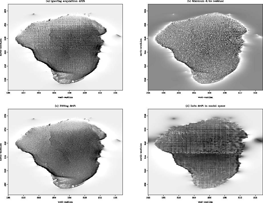
fig4
Figure 5
(a) Estimated  without attenuation of the tracks, i.e., equation ().
(b) Estimated with the derivative along the tracks, i.e., equation ().
(c) Estimated without tracks, i.e., equation ().
(d) Recorder drift in model space
without attenuation of the tracks, i.e., equation ().
(b) Estimated with the derivative along the tracks, i.e., equation ().
(c) Estimated without tracks, i.e., equation ().
(d) Recorder drift in model space  .
.


 fig4b
fig4b
Figure 6 Close-ups of the western
shore of the Sea of Galilee.
(a) Estimated without attenuation of the tracks, i.e., equation ().
(b) Estimated with the derivative along the tracks, i.e., equation ().
(c) Estimated without tracks, i.e., equation ().
(d) Recorder drift in model space .
Figures a and c display a comparison of the
estimated with or without the attenuation of the vessel
tracks. It is delightful that Figure c is
essentially track-free without any loss of details compared to Figure
a. The difference plot in Figure
d between the two results corroborates this and
does not show any geological feature. A close-up of Figure
is displayed in Figure . The differences
between the proposed techniques are clearly visible.
Comparing Figure c and Figure b,
we see that the drift-modeling strategy [equation ]
works much better than the noise-filtering strategy [equation
]. One possible explanation for
the difference between the two results is that the modeling approach is
more adaptive than the filtering of the residual. Indeed, by
introducing the modeling operator, we basically look for
the best that models the drift of the data on each track at
each point. The price to pay is an increase of the number of unknowns in equation
(). The reward is a surgically removed acquisition
footprint. Notice that we can identify the ancient shorelines in the
west and east parts of the lake very well.
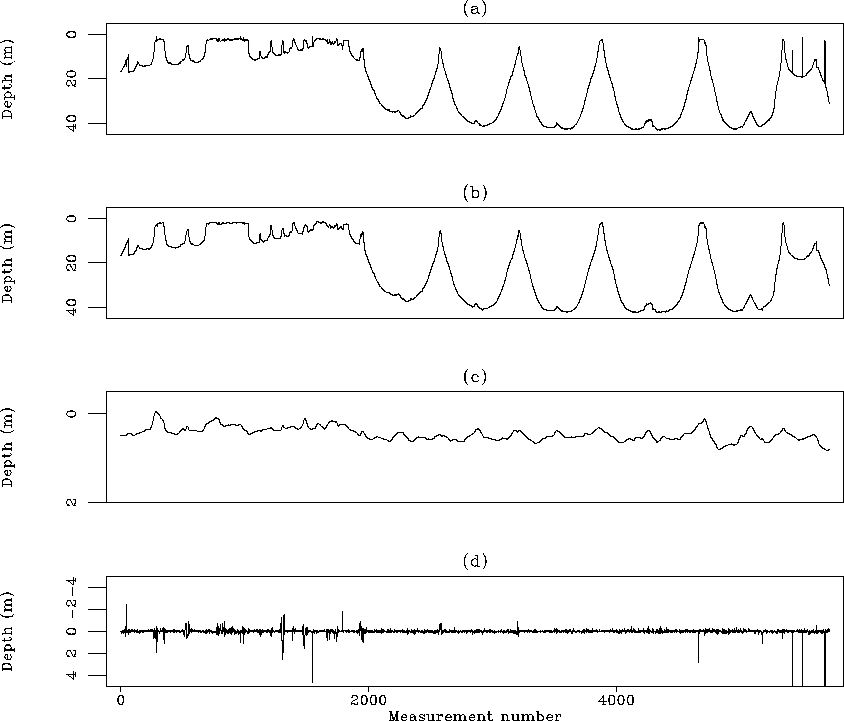
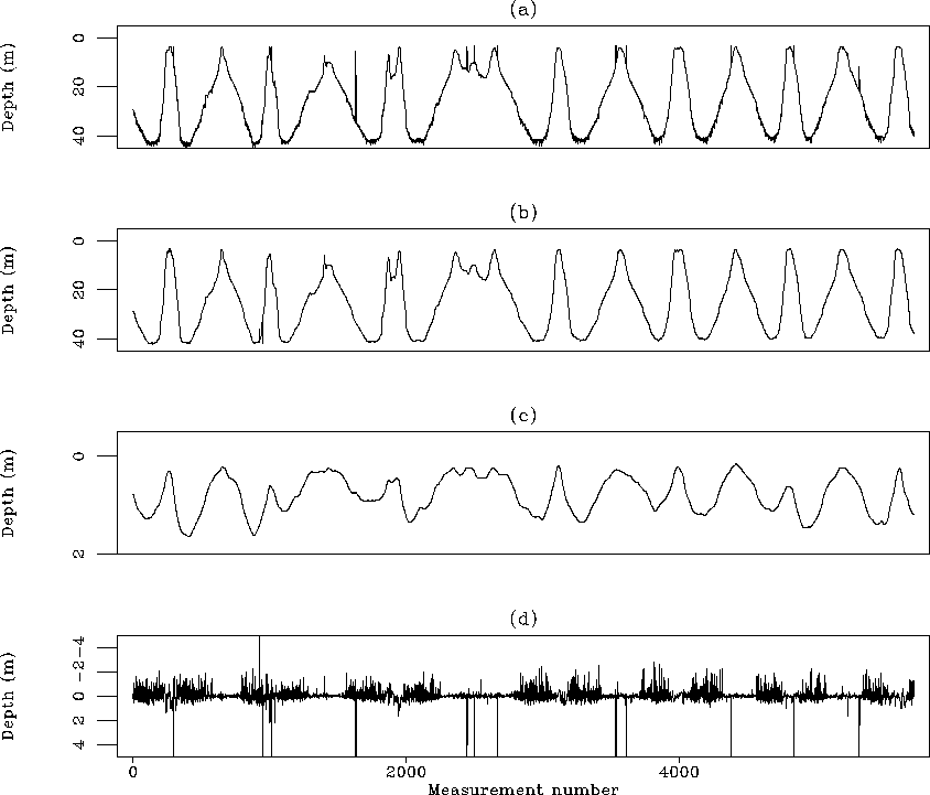
To better understand what is done, Figures
and show some segments of
the input data (), the estimated noise-free data ( ), the estimated secular variations (
 ) and the residual (
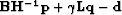 ) after inversion.
The estimated noise-free data in Figures b and
b show no remaining spikes. The effect of the
track attenuation is more difficult to see because the amplitude of
the drift is much smaller than the amplitude of the measurements.
Notice in Figure c that the estimated drift seems to
have reasonable amplitudes: the average drift is around 15 cm for
an accuracy of about 10 cm for the measurements.
We also observe that the estimated drift is relatively constant
throughout Figure c.
Now, looking at the estimated drift for another portion of
the data (Figure c),
notice that the drift has more variance than in Figure
c and oscillates between
0 to 2 m, which is too much. In addition, the estimated drift seems to follow the
bathymetry of the lake in Figure a.
Decreasing would attenuate the drift component with
the effect of increasing the tracks in the final image, however.
) after inversion.
The estimated noise-free data in Figures b and
b show no remaining spikes. The effect of the
track attenuation is more difficult to see because the amplitude of
the drift is much smaller than the amplitude of the measurements.
Notice in Figure c that the estimated drift seems to
have reasonable amplitudes: the average drift is around 15 cm for
an accuracy of about 10 cm for the measurements.
We also observe that the estimated drift is relatively constant
throughout Figure c.
Now, looking at the estimated drift for another portion of
the data (Figure c),
notice that the drift has more variance than in Figure
c and oscillates between
0 to 2 m, which is too much. In addition, the estimated drift seems to follow the
bathymetry of the lake in Figure a.
Decreasing would attenuate the drift component with
the effect of increasing the tracks in the final image, however.
Looking closely at the residual (Figure d), the drift
is large where the data are noisy (Figure a).
It is possible that the day of acquisition was very windy, which is
not a rare weather condition for the Sea of Galilee Volohonsky et al. (1983).
Thus, the wind forces the water to pile-up on one
side of the lake which can explain the lower water level on the other
side. A rapid calculation shows that the seiche period for the Sea
of Galilee is roughly 40 mn (assuming a lake length of 20 km and an
average depth of 30 m), which is well within a day of data acquisition.
In addition, the strong wind in the middle of the lake induces noisy
measurements because of the waves and of the erratic movement of the
ship. It is also possible that the depth sounder was not working
properly that day and had problems to correctly measure the deepest
part of the lake. These causes could probably explain
the shape and amplitude of the estimated drift in Figure
c, but we can't be absolutely sure.
It is very unfortunate that no daily logs of the survey
were kept in order to better interpret these results, especially
for such a noisy dataset.
fig5
Figure 7
(a) Input data acquired between A1 and B1 in Figure .
The ship is approximately moving bottom to top going east from A1 to B1.
(b) estimated after inversion, i.e., the estimated noise-free data.
(c) Estimated drift after inversion.
(d) Data residual after inversion.
The horizontal axis represents the measurement number.
fig6
Figure 8
(a) Input data acquired between A2 and B2 in Figure .
The ship is approximately moving right to left going south from A2 to B2.
(b) estimated after inversion, i.e., the estimated noise-free data.
(c) Estimated drift after inversion.
(d) Data residual after inversion.
The horizontal axis represents the measurement number.
Next: Conclusion
Up: Attenuation of the ship
Previous: Abandoned strategy for attenuating
Stanford Exploration Project
5/5/2005